
Projectile Motion
Objectives
-
•to test the validity of the kinematics model for simple projectile motion
Equipment
- inclined plane
- guided track
- Science Workshop interface
- photogates
- Time-of-Flight Accessory
- lab jack
- ball
- metric ruler
- plumb bob
- masking tape
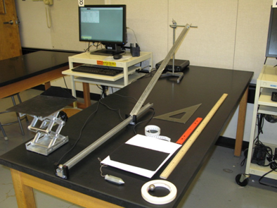
Figure 1
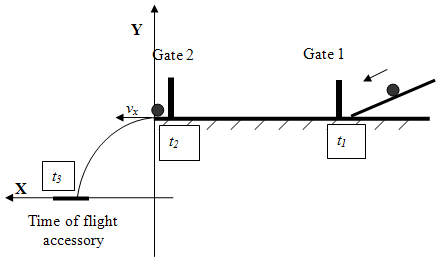
Figure 2: The experimental setup for Projectile Motion lab
Introduction and Theory
Consider the projectile motion of a ball as shown in fig. 3. At t = 0, the ball is released at the position specified by coordinates (0, y0) with horizontal velocity vx. The object moves with constant velocity in the horizontal direction. The horizontal range of its motion can be found with the equation of motion used to describe constant velocity motion.( 1 )
x = vxt
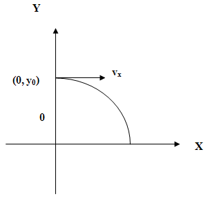
Figure 3: The system of coordinates for the projectile's motion.
( 2 )
y = y0 + v0yt +
gyt2
| 1 |
| 2 |
( 3 )
v = v0y + gyt,
x = vxt
), (2y = y0 + v0yt +
gyt2
| 1 |
| 2 |
v = v0y + gyt,
) describes a kinematics model for projectile motion launched horizontally.
An object launched horizontally has a zero initial velocity in vertical direction (v0y = 0). Thus, the equations (2y = y0 + v0yt +
gyt2
| 1 |
| 2 |
v = v0y + gyt,
) can be simplified.
( 4 )
y = y0 +
gyt2
| 1 |
| 2 |
( 5 )
vy = gyt
Procedure
Please print the worksheet for this lab. You will need this sheet to record your data.
Caution:
When taking measurements with the Time-of-Flight Accessory, keep it in place by hand, otherwise it will move on impact with the ball.
When taking measurements with the Time-of-Flight Accessory, keep it in place by hand, otherwise it will move on impact with the ball.
1
Mark the release position of the ball on the inclined V-shape track using the masking tape.
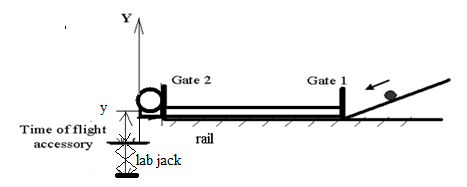
Figure 4
2
Hang the plumb bob from the launch point straight down to the floor and mark that point on the floor with the masking tape. Fasten the measuring tape to the floor. The tape will be used to measure the distance from the launch point to the lab jack. Be sure to line up the zero with the launching point marked on the floor.
3
Measure and record the height (h) from the bottom of the ball, when it is placed at the end of the guided track to the floor.
4
From the marked position on the v-track, launch the ball a couple of times to estimate the landing position of the projectile. Place the lab jack at the landing point. Attach the Time-of-Flight Accessory to the metal plate on the lab jack using the double-sticky tape.
5
Bring the lab jack to the lowest height setting, and record the height of the lab jack (h1) from the floor.
Caution:
The Time-of-Flight Accessory is a very delicate device - handle it with care.
The Time-of-Flight Accessory is a very delicate device - handle it with care.
6
Fold a piece of plain paper in half from the portrait orientation ("hamburger style") and place the black side of the carbon paper face down onto the top of the folded plain paper.
7
Open the pre-set experiment file: Labs/PHY 113/PreSetUp Labs/Projectile motion. Data Studio will record time intervals t12 (Column 1) and t23 (Column 2) as well as the initial horizontal velocity (vx) of the projectile object (Column 3).
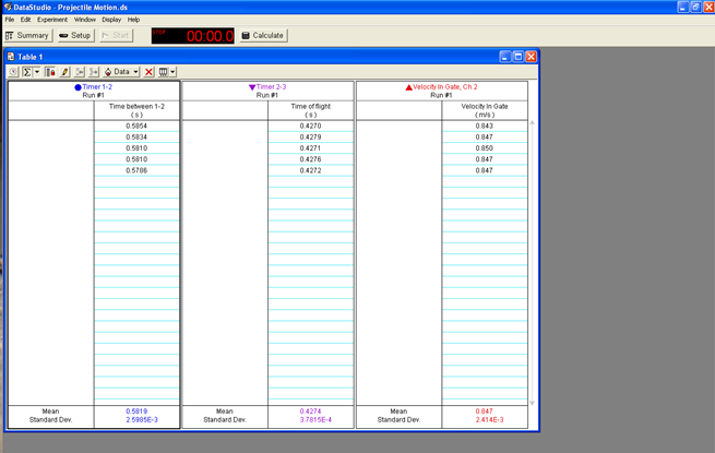
Figure 5
8
Open GA. Create 5 Manual Columns: Height (m), Xmin (m), Xmax (m), t23mean (s), Vmean (m/s). Create 3 calculated columns: Xexperimental, t23corr, (t23corr)2. The equations are provided in Appendix A.
9
Press "Start" and let the ball roll and land on the Time-of-Flight Accessory. Hold the Time-of-Flight Accessory to prevent its movement during the impact. Without stopping the recording, bring the ball back to the same release point and repeat the measurements four more times. Each time the ball passes through the photogates and hits the Time-of-Flight plate, a new row of data is added to the table. After all five runs are completed, to finish collecting one data set, press "Stop".
10
Type into the GA the t23mean value and Vmean recorded by the Data Studio.
11
Use the cluster of positions recorded on the paper placed on the Time-of-Flight Accessory to calculate the experimental value of the horizontal range and its error. Measure (Xmin) the distance from the launch point to the closest point of impact. Measure (Xmax) the distance from the launch point to the farthest point of impact. The equation provided in Appendix A needs to be used to calculate the mean value of the experimental horizontal range, xexperimental,
and its error, Δxexperimental.
Hint: To measure the experimental horizontal range between the edge of the Time-of-Flight Accessory to the closest and farthest points of impact, use the 30-cm ruler. Add this distance to the distance from the launch point to the lab jack measured with the measuring tape fastened to the floor.
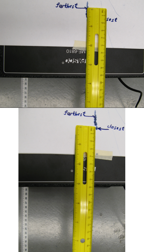
Figure 6: The top image is (9.4 + 30.5) cm for the farthest point. The bottom image is (7.9 + 30.5) cm for the closest point.
12
Five more times repeat step 9 -11 with a different lab jack height by changing and recording the height of the lab jack (like in step 5) for each trial.
You should have data for a total of 6 trials.
Data Analysis
NOTE: Use the equations provided in Appendix A and in the Introduction and Theory section to complete the Data Analysis.
1
In Graphical Analysis, build a graph: (X(experimental)-range vs t23corr). Apply linear fit to find the launched theoretical velocity, vtheo, and its uncertainty using the slope of the graph and its uncertainty.
2
In GA, choose - Insert - Graph. Plot Vmean vs Vmean graph, and then click STAT

Figure 7
3
Calculate the percent discrepancy between the experimental, Vmean-exp, and theoretical, vtheo, values of the launched velocity.
4
In GA, choose - Insert - Graph. Plot a graph: (height vs (t23corr)2). Apply linear fit. Use the slope of the graph to calculate the free fall acceleration, gexp, and its uncertainty.
5
Calculate the percent discrepancy between the experimental and theoretical values (gtheor = 9.81 m/s2)
The following calculations need to be done for only one of the runs.
6
Calculate the theoretical time-of-flight, ttheor, of the projectile ball using eqn 4y = y0 +
gyt2
| 1 |
| 2 |
7
Calculate the percent discrepancy between the corrected time of flight experimental for the chosen run and theoretical time-of-flight calculated above.
8
Using the corrected time-of-flight experimental, t23corr, and the experimental value of the launched velocity, Vmean, compute the theoretical horizontal range of the projectile, xtheor,
and its error, Δxtheor,
for the chosen trials.
9
Calculate the percent discrepancy between the theoretical value of the horizontal range and the value of experimental horizontal ranges for the chosen trail from GA.
10
Knowing the corrected time-of-flight t23corr of the projectile, use eqn 4 y = y0 +
gyt2
| 1 |
| 2 |
11
Calculate the percent discrepancy between the theoretical and the experimental value of the height of the projectile for the chosen trial.
Discussion
State the purpose of the lab. Based on your calculations for physics quantities – free fall acceleration, height, horizontal range, and launched velocity – do all of the experimental results fit within the error the results predicted by the theory? What is the relationship between the horizontal range and elapsed time based on your experimental data? What is the relationship between the height and the elapsed time? What are the types of motion the projectile object experienced in horizontal and vertical direction? Do your experimental results confirm the validity of the set of equations used to describe a kinematics model for projectile motion launched horizontally? Any meaningful comparison should include the uncertainties. Discuss reasons for any substantial discrepancies between experimental and theoretical results. What is the source of statistical and/or systematic error in this lab?Conclusion
-
•Have you met the objective of the Lab "Projectile Motion"?
-
•What major characteristics of the projectile motion have you proved with your experimental data?
Appendix A
( 6 )
Δttheor =
 |
| 1 |
| 2 |
 |
| ttheor × Δy |
| yexp |
( 7 )
t23corr = t23 −
d = 22 mm – the ball's diameter| d |
| Vmean |
( 8 )
Δt23corr =
− standard deviation of the mean of Δt23corr
| δt23 | ||
|

( 9 )
x theor = Vmean × t23corr
( 10 )
Δx theor = t23corr ×
+ v ×
| δv | ||
|
| δt23 | ||
|
( 11 )
x experimental =
| xmin + xmax |
| 2 |
( 12 )
Δx experimental =
| xmax − xmin |
| 2 |
( 13 )
Δytheor = gt23corr × Δt23corr