Lab 3 - Newton's Second Law

Introduction

Sir Isaac Newton put forth many important ideas in his famous book The Principia. His three laws of motion are the best known of these. The first law seems to be at odds with our everyday experience. Newton's first law states that any object at rest that is not acted upon by outside forces will remain at rest, and that any object in motion not acted upon by outside forces will continue its motion in a straight line at a constant velocity. If we roll a ball across the floor, we know that it will eventually come to a stop, seemingly contradicting the First Law. Our experience seems to agree with Aristotle's idea, that the "impetus" given to the ball is used up as it rolls. But Aristotle was wrong, as is our first impression of the ball's motion. The key is that the ball does experience an outside force, i.e., friction, as it rolls across the floor. This force causes the ball to decelerate (that is, it has a "negative" acceleration). According to Newton's second law an object will accelerate in the direction of the net force. Since the force of friction is opposite to the direction of travel, this acceleration causes the object to slow its forward motion, and eventually stop. The purpose of this laboratory exercise is to verify Newton's second law.

Discussion of Principles

Newton's second law in vector form is

( 1 )

	F

= ma

or F

_net = ma

This force causes the ball rolling on the floor to decelerate (that is, it has a "negative" acceleration). According to Newton's second law an object will accelerate in the direction of the net force. If

is the magnitude of the net force, and if

is the mass of the object, then the acceleration is given by

( 2 )

Since the force of friction is in the opposite direction to the direction of motion, this acceleration causes the object to slow its forward motion, and eventually stop. Notice that Eq. (1) and Eq. (2) are written in vector form. This means that Newton's second law holds true in all directions. You can always break up the forces and the resultant acceleration into their respective components in the

, and

directions.

( 3 )

F_net,x = ma_x

( 4 )

F_net,y = ma_y

( 5 )

F_net,z = ma_z

Consider a cart on a low-friction track as shown in Fig. 1. A light string is attached to the cart and passes over a pulley at the end of the track and a second mass is attached to the end of this string. The weight of the hanging mass provides tension in the string, which helps to accelerate the cart along the track. A small frictional force will resist this motion. We assume that the string is massless (or of negligible mass) and there is no friction between the string and the pulley. Therefore the tension in the string will be the same at all points along the string. This results in both masses having the same magnitude of acceleration but the direction of the acceleration will be different. The cart will accelerate to the right while hanging mass will accelerate in the downward direction as shown in Fig. 1.

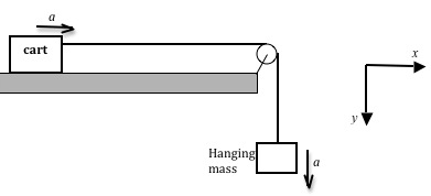
Figure 1: Two-mass System

We will take the positive direction to be in the direction of the acceleration of the two masses as indicated by the coordinate axes system in Fig 1. The free-body diagrams for the two masses are shown in Fig. 2. Let's look at the forces acting on each mass.

Figure 2: Free-body diagrams for the two masses

For the falling mass

m₁

, there are no forces acting in the horizontal direction. In the vertical direction it is pulled downward by gravity giving the object weight,

W = m₁g

and upward by the tension

in the string. See Fig. 2b. Thus Newton's second law applied to the falling mass in the

direction will be

( 6 )

F_net,1 = m₁g − T = m₁a

where the downward direction has been chosen to be positive. Figure 2a shows the forces acting on

m₂

. There is no motion of the cart in the vertical direction. Therefore the net force in the vertical direction will be zero, as will the acceleration. In the horizontal direction, the tension in the string acts in the

direction on the cart while the friction force between the cart's tires and the surface of the track acts in the

−x

direction. Newton's second law, in the

and

directions, respectively, are

( 7 )

F_net,2x = T − f = m₂a

( 8 )

F_net,2y = F_N − m₂g = 0

Since the cart and the hanging mass are connected by the string, which does not stretch, both accelerations appearing in Eq. (6) and Eq. (7) represent the same physical qualities. The tensions are the same due to Newton's third law. Combine Eq. (6) and Eq. (7) to eliminate

( 9 )

m₁g = (m₁ + m₂)a + f

Note that Eq. (9) has the form of a linear equation

y = mx + b

, where m is the slope and

is the

-intercept.

Objective

The objective of this experiment is to verify the validity of Newton's second law, which states that the net force acting on an object is directly proportional to its acceleration. Eq. (9) was derived on the basis of this law. Therefore we can consider Eq. (9) to be a prediction of the second law. In this experiment we will seek to verify this specific prediction and thereby provide evidence for the validity of the second law.

Equipment

Low-friction track with pulley
Cart
String
Balance
DataStudio software
Two photogates
Assorted masses
Weight hanger
Computer
Signal interface

Procedure

You will conduct several trials, keeping the total mass

M = m₁ + m₂

constant while varying

m₁

and therefore

m₂

, to obtain a different value of

for each value of

m₁

. By graphing

versus

m₁g

you will be able to find

, the total mass of the system from Eq. (9). The cart has an attached metal flag that will cause two photogates placed a fixed distance apart to react as the cart passes through them. A computer connected to the photogate will measure and display the time intervals elapsing while the flag passes through the two photogates. From these time intervals and the length of the flag, the computer will calculate the velocities

v₁

and

v₂

of the cart at each of the photogates. Additionally, from the computer data you can determine the time interval

Δt

it takes for the cart to travel between the photogates. The acceleration

between the two gates can then be calculated from

( 10 )

a =

v₂ − v₁

Δt

where

v₁

is the velocity at the first photogate, and

v₂

is the velocity at the second photogate.

Setting up the equipment

Using the adjusting screws underneath level the track so that the cart does not move when placed by itself in the center of the track. Since the cart has some friction, test to see if the track is level by giving the cart a slight nudge to the right and comparing the motion with a similar push to the left.

Place the photogates sufficiently far apart. Make sure the cart's flag is before the first gate when the hanger is all the way up near the pulley as shown in Fig. 3a. Also, make sure the cart's flag passes the second photogate before the hanger hits the ground. See Fig. 3b. This will ensure that the cart is being accelerated in the region between the two photogates.

Adjust the height of each photogate so that the small metal flag on the cart blocks the photogate light beam as it passes.

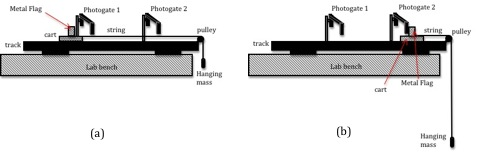
Figure 3: Photogate set-up

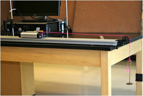
Figure 4: Experimental set-up

Connect photogate 1 to digital channel 1 and photogate 2 to digital channel 2. If the photogates are plugged in properly, the red LED on the photogate will light up when the infrared beam is blocked.

Open the appropriate Capstone file associated with this lab. Fig. 5 shows the opening screen in Capstone.

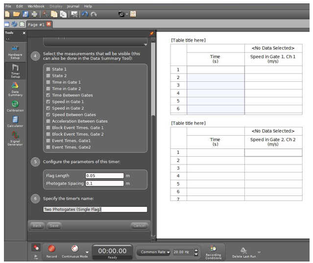
Figure 5: Newton's second law display

The length of the small metal flag on the cart is different for each cart. Measure for your cart and record it on the worksheet.

You must input the value of the flag length and the spacing between photogates, as shown in Fig. 6. Remember to click on the Save button.

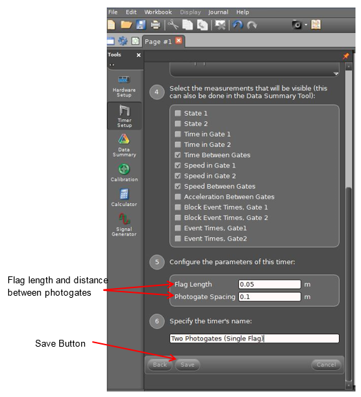
Figure 6: Entering the flag length

Data Aquisition

Place the cart at the end of the track away from the pulley. Add three 50-gram masses to the cart.

Weigh the weight hanger, and record the mass

M_h

on the worksheet.

Connect one end of the string to the weight hanger and the other end to the cart, placing the string over the pulley. See Fig. 3.

Hold the cart in position so that the cart will accelerate when released. When ready to record data, click the Start button. Release the cart and catch it when it reaches the end of the track. Click the Stop button to end data recording. The time and speed data for each photogate will be reported automatically in the Table. See Fig. 7.

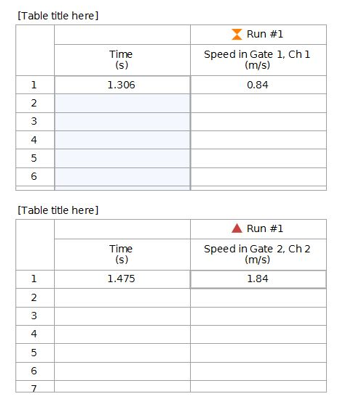
Figure 7: Sample data table

The cart's speed increases smoothly during the time interval while the flag passes through the photogate beam. At some instant during that time interval the cart's instantaneous speed equals the average speed for the interval. That instant of time is shown in the "Time (s)" column next to its associated velocity.

The time it took for the cart to travel between photogates 1 and 2 is

Δt

. This is calculated by subtracting the time value in the column labeled Velocity in Gate, Ch1 from the time value in the column labeled Velocity in Gate, Ch 2. Calculate

Δt

and record this in Data Table 1 on the worksheet.

Use this time interval together with the two velocities

v₁

and

v₂

in Eq. (10) to calculate the acceleration of the cart between the two photogates and record this result in Data Table 1.

Move one 50-gram mass from the cart to the weight hanger. Note: You must keep the total mass constant, so any mass removed from the cart must be added to the weight hanger.

Repeat steps 11 through 15 three more times, until you have a total of four runs with a different value of the hanging mass for each run. Calculate and record the acceleration for each case.

Checkpoint 1:
Ask your TA to check your table values before proceeding.

Analyzing the Results

Using Excel plot

m₁g

versus

. See Appendix G.

Use the trendline option in Excel to draw a best fit line to the data and determine the slope and

-intercept. See Appendix H. Record these values on the worksheet.

From the value of the slope determine the total mass of the system.

Use a balance to measure the mass of the cart. Add this to the mass of the weight hanger and the added masses to find the total mass

of the system.

Compare this measured mass to the mass determined from the slope of the graph by calculating the percent difference. Record this on the worksheet. See Appendix B.

Checkpoint 2:
Ask your TA to check your Excel worksheet and graph.