
Lab 4 - Conservation of Mechanical Energy
Introduction
When a body moves, some things—such as its position, velocity, and momentum—change. It is interesting and useful to consider things that do not change. The total energy is a quantity that does not change; we say that it is conserved during the motion. There are several forms of energy with which you may be familiar, such as solar, nuclear, electrical, and thermal energies. In this experiment you will investigate two kinds of mechanical energy: kinetic energy and potential energy. You will carry out an experiment that demonstrates the conservation of the total mechanical energy of a system.Discussion of Principles
Conservation of Mechanical Energy
The total mechanical energyE
of a system is defined as the sum of the kinetic energy K
and potential energy U
of the system.
( 1 )
E = K + U
K1
, U1
, K2
, U2
are the kinetic and potential energies at two different locations 1 and 2 respectively, then the conservation of mechanical energy leads to the following mathematical expression
( 2 )
K1 + U1 = K2 + U2
( 3 )
ΔK + ΔU = 0
ΔK = K2 − K1
and ΔU = U2 − U1
.
Conservation of Mechanical Energy is one of the fundamental laws of physics that is also a very powerful tool for solving complex problems in mechanics.
Kinetic Energy
Kinetic energyK
is the energy a body has because it is in motion. When work is done on an object, the result is a change in the kinetic energy of the object. Energy of motion can be translational kinetic energy and/or rotational kinetic energy.
Translational kinetic energy KT
is the energy an object has because it is moving from place to place, regardless of whether it is also rotating; KT
is related to the mass m
and velocity or speed v
of the object by
( 4 )
KT =
mv2
| 1 |
| 2 |
KR
is the energy an object has because it is rotating, regardless of whether the body as a whole is moving from place to place. KR
is related to the moment of inertia I
and angular velocity ω
of the object by
( 5 )
KR =
I ω2
| 1 |
| 2 |
R
of the sphere.
( 6 )
ω =
| v |
| R |
m
of a body is a measure of its resistance to a change in its (translational) velocity, the moment of inertia I
of an object is a measure of that object's resistance to a change in its angular velocity. The moment of inertia of a solid sphere (of uniform density) is given by
( 7 )
I =
MR2
| 2 |
| 5 |
M
and R
are the mass and radius of the sphere, respectively.
The total kinetic energy Ktotal
of the rolling sphere used in this experiment is the sum of the translational and rotational kinetic energies.
( 8 )
Ktotal = KT + KR
Potential Energy
An object might have energy by virtue of its position on account of the work done to put it there. The object is said to have potential energyU
. Gravitational potential energy, which we will be concerned with in this experiment, depends on the mass of the object, the acceleration due to gravity, and its location. It is important to remember that potential energy is only defined relative to a location, which can be chosen arbitrarily (that is, for convenience) without affecting the body's subsequent motion. For example, if the rolling sphere is held 1/2 meter above a table top, and the table top is 1 meter above the floor, the potential energy of the sphere has one value relative to the table top and a larger value relative to the floor.
The potential energy of an object near the surface of the Earth is given by
( 9 )
U = mgh
g
is the acceleration due to gravity, m
is the mass of the object, and h
is the height above the chosen reference level (the end of the ramp, where the potential energy is zero by choice).
If we drop an object, it will lose height and gain velocity as it falls in accordance with Eq. (2)K1 + U1 = K2 + U2
.
Objective
The objective of this experiment is to determine if the law of conservation of mechanical energy can predict the velocity of a rolling sphere after rolling down a ramp. You will test your hypothesis by placing the sphere at various heights and measuring the velocity at the end of the ramp. You will compare the measured velocity with the predicted velocity using the conservation of mechanical energy. If we let the sphere roll down a ramp, its vertical height will decrease while its translational and rotational velocity will increase. Potential energy is lost and kinetic energy is gained. Assuming that the sphere rolls without slipping and there is no friction or air drag, the loss of potential energy will equal the gain in kinetic energy. Based on conservation of mechanical energy, if the sphere is placed at heighth1
, as shown in Fig. 1, you can show that the final speed v2
at the end of the ramp is
( 10 )
v2 =
 |
|
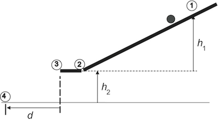
Figure 1: Sphere rolling down a ramp
v2 =
tells us that we can predict the final translational speed |
|
v2
of the sphere at point  at the bottom of the inclined portion of the ramp if we know the initial height
 h1
.
In the experiment you will measure the translational speed of the sphere at the bottom of the ramp and compare it to the speed predicted by the conservation of mechanical energy. If these two (experimental and predicted) values of the translational speed are in close agreement, you can say that you have verified the law of conservation of mechanical energy.
Experimental Design
Let us consider several ways in which the translational speed of a small sphere can be measured.-
1Use a police radar speed gun: A radar gun or speed gun is a small Doppler radar unit used to detect the speed of objects, especially trucks and automobiles for the purpose of regulating traffic, as well as pitched baseballs, runners or other moving objects in sports. It relies on the Doppler Effect applied to a radar beam to measure the speed of objects at which it is pointed. Radar guns may be hand-held or vehicle-mounted; see "Radar gun" or "Police RADAR". A radar speed gun measures the instantaneous speed of the sphere. As the sphere rolls down the ramp, its speed changes. It would be difficult to read the radar gun at the precise moment when the small sphere reaches the bottom of the ramp.
-
2Use an ultra sonic motion detector: The sonic motion detector transmits a burst of ultrasonic pulses. The ultrasonic pulses reflect off a target and return to the face of the sensor. The target indicator flashes when the transducer detects an echo. The sensor measures the time between the trigger rising edge and the echo rising edge. It uses this time and the speed of sound to calculate the distance to the object. To determine velocity, it uses consecutive position measurements to calculate the rate of change of position. See, for example, PASCO or Vernier. In general, a sonic motion detector used in a physics lab can only detect objects no smaller than a baseball. Measuring the speed of a small steel marble would be unreliable.
-
3Use a photogate: A photogate monitors the motion of objects passing through its gate, counting events as the object breaks the infrared beam. If the size of the object is known, by measuring the time an object blocks the gate, you can determine the velocity. See, for example, Vernier or PASCO. The size of the infrared beam from a photogate is not small compared to the diameter of the sphere. Thus you could not make an accurate determination of the length passing through the infrared beam.
-
4Use kinematics: Once the sphere leaves the ramp, it is under free fall. By measuring the vertical and horizontal components of the sphere's displacement after it leaves the ramp, you can determine the sphere's speed at the end of the ramp. Measuring the horizontal and vertical displacements of the sphere does not involve the use of motion detectors or photogates and is straight forward. You will use this method for the experiment.
Finding the speed using kinematics
The ramp has a short horizontal section from point to point  . We assume that the sphere's speed down the ramp does not change when it travels on the short horizontal section between point and point . Once the sphere leaves the ramp, there is no force acting on it to change its horizontal velocity (assuming there is no air resistance). Gravity pulls the sphere down the instant it leaves the ramp. We will consider the equations of motion for the vertical and horizontal motions of the sphere.
The vertical distance
. We assume that the sphere's speed down the ramp does not change when it travels on the short horizontal section between point and point . Once the sphere leaves the ramp, there is no force acting on it to change its horizontal velocity (assuming there is no air resistance). Gravity pulls the sphere down the instant it leaves the ramp. We will consider the equations of motion for the vertical and horizontal motions of the sphere.
The vertical distance h2
that the sphere falls in time ΔT
is given by
( 11 )
h2 =
g(ΔT)2
| 1 |
| 2 |
g
= 9.81 m/s2 is the acceleration due to gravity. The initial vertical component of the velocity of the sphere as it leaves the ramp is zero.
The horizontal distance d
the sphere moves from the end of the ramp to the point where it touches the table is given by
( 12 )
d = v2(ΔT)
( 13 )
v2kinematics = d
|
|
Equipment
- Inclined ramp clamped to a table
- Small steel sphere
- Meter stick
- Carbon paper
- Bubble level
Procedure

h1
, allow it to roll down the ramp and read the distance d
from the edge of the ramp to the location where it hits the table.
Independently, you will make a graph of the horizontal velocity v2
versus horizontal distance d
using Eq. (13)v2kinematics = d
. From this graph you can read the horizontal velocity knowing the horizontal distance the sphere traveled for the 5 different vertical heights.
From your measurements of the horizontal and vertical distances that the sphere travels after leaving the end of the ramp, you will determine the experimental velocity for the 5 different vertical heights using Eq. (13) |
|
v2kinematics = d
and check these values with your graph.
|
|
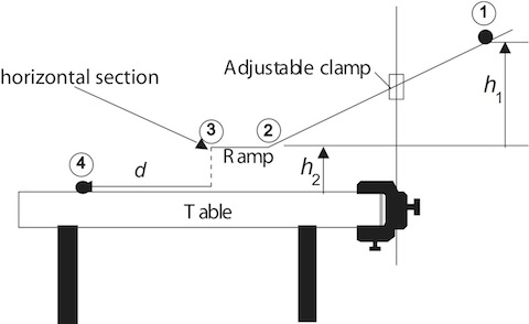
Figure 2: Schematic diagram of the apparatus.
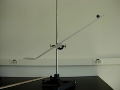
Figure 3: Actual apparatus.
Setting up
1
Tape several pieces of notebook paper to the top of the table, extending out from the edge of the horizontal section of the ramp to about 1 m. Set the ramp so that it rests on the paper, so that h2 = 0
. Mark the position of the lower edge of the ramp on the paper.
2
Adjust the ramp so that the horizontal section is about 18 to 20 cm above the table.
The ramp should be adjusted so that the horizontal section of the ramp is level, as indicated, by placing a small bubble level there.
If the lower edge of the ramp is not level, ask your lab instructor for help with this adjustment. This will be position h2
of the ramp throughout the experiment.
Make sure that you do not disturb it while doing the experiment.
Procedure A: Determining the experimental velocity v2exp using kinematics
3
Using Eq. (13)v2kinematics = d
prepare a graph, using Excel, of the velocity |
|
v2kinematics
versus the horizontal distance d
for two values of d
(namely zero and 50 cm). You will use this graph to read the experimental velocity of the ball v2exp
. See Appendix G.
Checkpoint 1:
Ask your TA to check your Excel graph of
Ask your TA to check your Excel graph of
v2kinematics
vs. d
.
4
Mark 5 positions along the length of the ramp at intervals of about 2.5 cm.
These are the positions from which you will release the sphere.
Do not start too close to the bottom of the incline. Make sure these positions are evenly spaced.
5
Measure the height of these positions from the table top and determine the height h1
for each of these positions. Record them in the data table. This is the vertical distance that the sphere falls while rolling down the ramp.
6
Place a piece of carbon paper face down on top of the paper on the table.
Do not tape the carbon paper to the table or the white sheet of paper.
7
Place the sphere at the first position on the ramp, and release it.
Note: You should place the center of the sphere at this mark and release it! Be careful not to push it down the ramp.
8
Remove the carbon paper. You will see a small spot on the underlying paper marking the point where the sphere landed.
Measure and record the horizontal distance d
from the line drawn earlier marking the end of the ramp to the point of impact.
Once you have measured the position of the dot, draw an "X" through it, and label it so that you will be able to distinguish it from later marks.
Record this distance in Data Table 1 on the worksheet.
9
You will do three trials for the same value of h1
to get the average value of d
. Therefore, repeat the process two more times for the same release position of the sphere and record the horizontal distance again and then take the average of the three values of d
. Record these values in Data Table 1.
10
Repeat steps 7 through 9 for each value of h1
by releasing the sphere from the positions you marked on the incline.
You might have to move the carbon paper out farther as the point of release goes further up the ramp. Label the impact points as they are produced so you do not get confused with marks made later.
Note: For each value of h1
you should have three trials from which you will find the average value of the horizontal distance d
.
11
For each height h1, use Eq. (13)v2kinematics = d
to determine |
|
v2exp
, the velocity of the sphere as it leaves the ramp.
Use the graph (see step 3) to verify your value of v2exp
.
Checkpoint 2:
Ask your TA to check your calculations before proceeding.
Ask your TA to check your calculations before proceeding.
Procedure B: Using the Conservation of Mechanical Energy to predict the velocity v2CME
12
For each of the 5 values of h1
that you used in procedure A, calculate the horizontal velocity v2CME
using conservation of mechanical energy as given by Eq. (10)v2 =
. Enter these values in data table 2.
|
|
13
Compute the percent difference between v2exp
and v2CME
for each value of h1
and record these in data table 2. See Appendix B.
Checkpoint 3:
Ask your TA to check your calculations.
Ask your TA to check your calculations.