Lab 7 - Simple Harmonic Motion

Introduction

Have you ever wondered why a grandfather clock keeps accurate time? The motion of the pendulum is a particular kind of repetitive or periodic motion called simple harmonic motion, or SHM. The position of the oscillating object varies sinusoidally with time. Many objects oscillate back and forth. The motion of a child on a swing can be approximated to be sinusoidal and can therefore be considered as simple harmonic motion. Some complicated motions like turbulent water waves are not considered simple harmonic motion. When an object is in simple harmonic motion, the rate at which it oscillates back and forth as well as its position with respect to time can be easily determined. In this lab, you will analyze a simple pendulum and a spring-mass system, both of which exhibit simple harmonic motion.

Discussion of Principles

A particle that vibrates vertically in simple harmonic motion moves up and down between two extremes y = ±A. The maximum displacement A is called the amplitude. This motion is shown graphically in the position-versus-time plot in Fig. 1.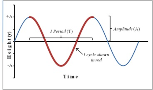

Figure 1: Position plot showing sinusoidal motion of an object in SHM

One complete oscillation or cycle or vibration is the motion from, for example,

y = −A

y = +A

and back again to

y = −A.

The time interval T required to complete one oscillation is called the period. A related quantity is the frequency f, which is the number of vibrations the system makes per unit of time. The frequency is the reciprocal of the period and is measured in units of Hertz, abbreviated Hz;

1 Hz = 1 s⁻¹.

( 1 )

f = 1/T

If a particle is oscillating along the y-axis, its location on the y-axis at any given instant of time t, measured from the start of the oscillation is given by the equation

( 2 )

y = A sin(2πft)

Recall that the velocity of the object is the first derivative and the acceleration the second derivative of the displacement function with respect to time. The velocity v and the acceleration a of the particle at time t are given by

( 3 )

v = 2πfA cos(2πft)

( 4 )

a = −(2πf)²[A sin(2πft)]

Notice that the velocity and acceleration are also sinusoidal. However the velocity function has a 90° or π/2 phase difference while the acceleration function has a 180° or π phase difference relative to the displacement function. For example, when the displacement is positive maximum, the velocity is zero and the acceleration is negative maximum. Substituting from Eq. (1) into Eq. (4) yields

( 5 )

a = −4π²f²y

From Eq. (5) we see that the acceleration of an object in SHM is proportional to the displacement and opposite in sign. This is a basic property of any object undergoing simple harmonic motion. Consider several critical points in a cycle as in the case of a spring-mass system in oscillation. A spring-mass system consists of a mass attached to the end of a spring that is suspended from a stand. The mass is pulled down by a small amount and released to make the spring and mass oscillate in the vertical plane. Figure 2 shows five critical points as the mass on a spring goes through a complete cycle. The equilibrium position for a spring-mass system is the position of the mass when the spring is neither stretched nor compressed.

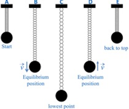
Figure 2: Five key points of a mass oscillating on a spring.

The mass completes an entire cycle as it goes from position A to position E. A description of each position is as follows:

Position A: The spring is compressed; the mass is above the equilibrium point at
y = A
and is about to be released.
Position B: The mass is in downward motion as it passes through the equilibrium point.
Position C: The mass is momentarily at rest at the lowest point before starting on its upward motion.
Position D: The mass is in upward motion as it passes through the equilibrium point.
Position E: The mass is momentarily at rest at the highest point before starting back down again.

By noting the time when the negative maximum, positive maximum, and zero values occur for the oscillating object's position, velocity, and acceleration, you can graph the sine (or cosine) function. This is done for the case of the oscillating spring-mass system in the table below and the three functions are shown in Fig. 3. Note that the positive direction is typically chosen to be the direction that the spring is stretched. Therefore, the positive direction in this case is down and the initial position A in Fig. 2 is actually a negative value. The most difficult parameter to analyze is the acceleration. It helps to use Newton's second law, which tells us that a negative maximum acceleration occurs when the net force is negative maximum, a positive maximum acceleration occurs when the net force is positive maximum and the acceleration is zero when the net force is zero.

	Position	Velocity	Acceleration
Point A	neg max	zero	pos max
Point B	zero	pos max	zero
Point C	pos max	zero	neg max
Point D	zero	neg max	zero
Point E	neg max	zero	pos max

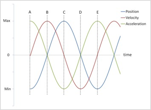
Figure 3: Position, velocity and acceleration vs. time

For this particular initial condition (starting position at A in Fig. 2), the position curve is a cosine function (actually a negative cosine function), the velocity curve is a sine function, and the acceleration curve is just the negative of the position curve.

Mass and Spring

A mass suspended at the end of a spring will stretch the spring by some distance y. The force with which the spring pulls upward on the mass is given by Hooke's law

( 6 )

F = −ky

where k is the spring constant and y is the stretch in the spring when a force F is applied to the spring. The spring constant k is a measure of the stiffness of the spring. The spring constant can be determined experimentally by allowing the mass to hang motionless on the spring and then adding additional mass and recording the additional spring stretch as shown below. In Fig. 4a the weight hanger is suspended from the end of the spring. In Fig. 4b, an additional mass has been added to the hanger and the spring is now extended by an amount

Δy

. This experimental set-up is also shown in the photograph of the apparatus in Fig. 5.

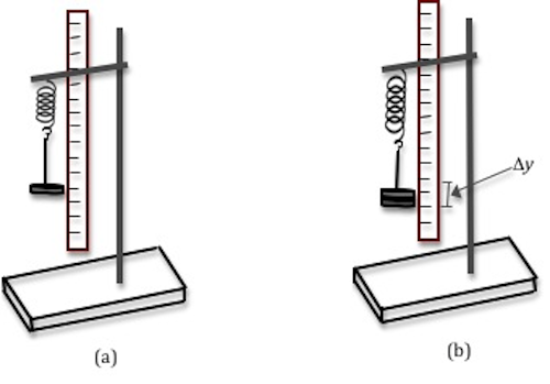
Figure 4: Set up for determining spring constant

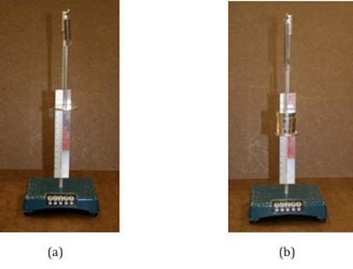
Figure 5: Photo of set-up for determining spring constant

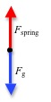
When the mass is motionless, its acceleration is zero. According to Newton's second law the net force must therefore be zero. There are two forces acting on the mass; the downward gravitational force and the upward spring force. See the free-body diagram in Fig. 6 below.

Figure 6: Free-body diagram for the spring-mass system

So Newton's second law gives us

( 7 )

Δmg − kΔy = 0

where

Δm

is the change in mass and

Δy

is the change in the stretch of the spring caused by the change in mass, g is the gravitational acceleration, and k is the spring constant. Eq. (7) can also be expressed as

( 8 )

Δm =

Δy

Newton's second law applied to this system is

ma = F = −ky.

Substitute from Eq. (5) for the acceleration to get

( 9 )

m(−4π²f²y) = −ky

from which we get an expression for the frequency f and the period T.

( 10 )

f =

2π

( 11 )

T = 2π

Using Eq. (11) we can predict the period if we know the mass on the spring and the spring constant. Alternately, knowing the mass on the spring and experimentally measuring the period, we can determine the spring constant of the spring. Notice that in Eq. (11) the relationship between T and m is not linear. A graph of the period versus the mass will not be a straight line. If we square both sides of Eq. (11), we get

( 12 )

T² = 4π²

Now a graph of

T²

versus m will be a straight line and the spring constant can be determined from the slope.

Simple Pendulum

The other example of simple harmonic motion that you will investigate is the simple pendulum. The simple pendulum consists of a mass m, called the pendulum bob, attached to the end of a string. The length L of the simple pendulum is measured from the point of suspension of the string to the center of the bob as shown in Fig. 7 below.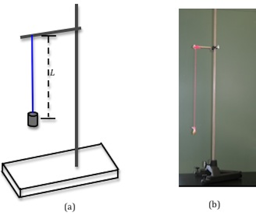

Figure 7: Experimental set-up for a simple pendulum

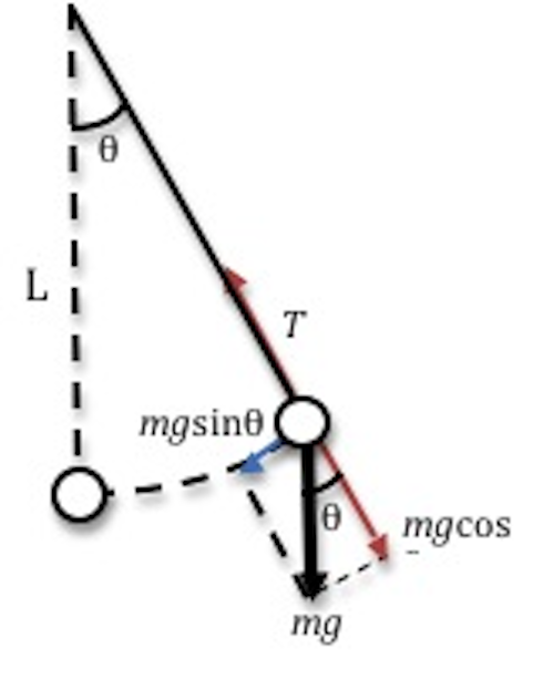
If the bob is moved away from the rest position through some angle of displacement θ as in Fig. 7, the restoring force will return the bob back to the equilibrium position. The forces acting on the bob are the force of gravity and the tension force of the string. The tension force of the string is balanced by the component of the gravitational force that is in line with the string (i.e. perpendicular to the motion of the bob). The restoring force here is the tangential component of the gravitational force.

Figure 8: Simple pendulum

When we apply trigonometry to the smaller triangle in Fig. 8, we get the magnitude of the restoring force

| = mg sin θ.

This force depends on the mass of the bob, the acceleration due to gravity g and the sine of the angle through which the string has been pulled. Again Newton's second law must apply, so

( 13 )

ma = F = −mg sin θ

where the negative sign implies that the restoring force acts opposite to the direction of motion of the bob. Since the bob is moving along the arc of a circle, the angular acceleration is given by

α = a/L.

From Eq. (13) we get

( 14 )

α = −

sin θ

In Fig. 9 the blue solid line is a plot of θ versus sin(θ) and the straight line is a plot of θ in degrees versus θ in radians. For small angles these two curves are almost indistinguishable. Therefore, as long as the displacement θ is small we can use the approximation sin θ ≅ θ.

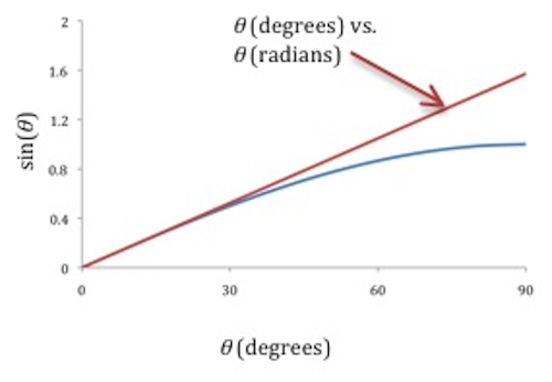
Figure 9: Graphs of sin θ versus θ

With this approximation Eq. (14) becomes

( 15 )

α = −

Equation (15) shows the (angular) acceleration to be proportional to the negative of the (angular) displacement and therefore the motion of the bob is simple harmonic and we can apply Eq. (5) to get

( 16 )

α = −4π²f² θ

Combining Eq. (15) and Eq. (16), and simplifying, we get

( 17 )

f =

2π

and

( 18 )

T = 2π

Note that the frequency and period of the simple pendulum do not depend on the mass.

Objective

The objective of this lab is to understand the behavior of objects in simple harmonic motion by determining the spring constant of a spring-mass system and a simple pendulum.

Equipment

Assorted masses
Spring
Meter stick
Stand
Stopwatch
String
Pendulum bob
Protractor
Balance

Procedure

Using Hooke's law you will determine the spring constant of the spring by measuring the spring stretch as additional masses are added to the spring. You will determine the period of oscillation of the spring-mass system for different masses and use this to determine the spring constant. You will then compare the spring constant values obtained by the two methods. In the case of the simple pendulum, you will measure the period of oscillation for varying lengths of the pendulum string and compare these values to the predicted values of the period.

Procedure A: Determining Spring Constant Using Hooke's Law

1
Starting with 50 g, add masses in steps of 50 g to the hanger. As you add each 50 g mass, measure the corresponding elongation y of the spring produced by the weight of these added masses. Enter these values in Data Table 1.
2
Use Excel to plot m versus y. See Appendix G.
3
Use the trendline option in Excel to determine the slope of the graph. Record this value on the worksheet. See Appendix H.
4
Use the value of the slope to determine the spring constant k of the spring. Record this value on the worksheet.

Checkpoint 1:
Ask your TA to check your table and Excel graph.

Procedure B: Determining Spring Constant from
T²
vs. m Graph

We have assumed the spring to be massless, but it has some mass, which will affect the period of oscillation. Theory predicts and experience verifies that if one-third the mass of the spring were added to the mass m in Eq. (11), the period will be the same as that of a mass of this total magnitude, oscillating on a massless spring.

5
Use the balance to measure the mass of the spring and record this on the worksheet. Add one-third this mass to the oscillating mass before calculating the period of oscillation. If the mass of the spring is much smaller than the oscillating mass, you do not have to add one-third the mass of the spring.
6
Add 200 g to the hanger.
7
Pull the mass down a short distance and let go to produce a steady up and down motion without side-sway or twist. As the mass moves downward past the equilibrium point, start the clock and count "zero." Then count every time the mass moves downward past the equilibrium point, and on the 50th passage stop the clock.
8
Repeat step 7 two more times and record the values for the three trials in Data Table 2 and determine an average time for 50 oscillations.
9
Determine the period from this average value and record this on the worksheet.
10
Repeat steps 7 through 9 for three other significantly different masses.
11
Use Excel to plot a graph of
T²
vs.
m
.
12
Use the trendline option in Excel to determine the slope and record this value on the worksheet.
13
Determine the spring constant k from the slope and record this value on the worksheet.
14
Calculate the percent difference between this value of k and the value obtained in procedure A using Hooke's law. See Appendix B.

Checkpoint 2:
Ask your TA to check your table values and calculations.

Procedure C: Simple Pendulum

15
Adjust the pendulum to the greatest length possible and firmly fasten the cord. With a 2-meter stick, carefully measure the length of the string, including the length of the pendulum bob. Use a vernier caliper to measure the length of the pendulum bob. See Appendix D. Subtract one-half of this value from the length previously measured to get the value of L and record this in Data Table 3 on the worksheet.
16
Using the accepted value of 9.81
m/s²
for g, predict and record the period of the pendulum for this value of L.
17
Pull the pendulum bob to one side and release it. Use as small an angle as possible, less than 10°. Make sure the bob swings back and forth instead of moving in a circle. Using the stopwatch measure the time required for 50 oscillations of the pendulum and record this in Data Table 3.
18
Repeat step 17 two more times and record the values for the three trials in Data Table 3 and determine an average time for 50 oscillations.
19
Determine the period from this average value and record this on the worksheet.
20
Calculate the percent error between this value and the predicted value of the period.
21
Repeat steps 16 through 20 for three other significantly different lengths.

Checkpoint 3:
Ask your TA to check your table values and calculations.