
Simple Harmonic Motion – Concepts
Introduction
Have you ever wondered why a grandfather clock keeps accurate time? The motion of the pendulum is a particular kind of repetitive or periodic motion called simple harmonic motion, or SHM. The position of the oscillating object varies sinusoidally with time. Many objects oscillate back and forth. The motion of a child on a swing can be approximated to be sinusoidal and can therefore be considered as simple harmonic motion. Some complicated motions like turbulent water waves are not considered simple harmonic motion. When an object is in simple harmonic motion, the rate at which it oscillates back and forth as well as its position with respect to time can be easily determined. In this lab, you will analyze a simple pendulum and a spring-mass system, both of which exhibit simple harmonic motion.Discussion of Principles
A particle that vibrates vertically in simple harmonic motion moves up and down between two extremes y = ±A. The maximum displacement A is called the amplitude. This motion is shown graphically in the position-versus-time plot in Figure 1.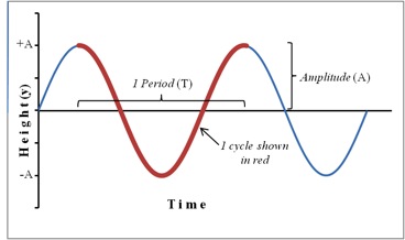
Figure 1: Position plot showing sinusoidal motion of an object in SHM
y = −A
to y = +A
and back again to y = −A.
The time interval T required to complete one oscillation is called the period. A related quantity is the frequency f, which is the number of vibrations the system makes per unit of time. The frequency is the reciprocal of the period and is measured in units of Hertz, abbreviated Hz; 1 Hz = 1 s−1.
If a particle is oscillating along the y-axis, its location on the y-axis at any given instant of time t, measured from the start of the oscillation is given by the equation
Recall that the velocity of the object is the first derivative and the acceleration the second derivative of the displacement function with respect to time. The velocity v and the acceleration a of the particle at time t are given by the following.
Notice that the velocity and acceleration are also sinusoidal. However, the velocity function has a 90° or π/2 phase difference while the acceleration function has a 180° or π phase difference relative to the displacement function. For example, when the displacement is positive maximum, the velocity is zero and the acceleration is negative maximum.
Substituting from equation 2 into equation 4 yields
From equation 5, we see that the acceleration of an object in SHM is proportional to the displacement and opposite in sign. This is a basic property of any object undergoing simple harmonic motion.
Consider several critical points in a cycle as in the case of a spring-mass system in oscillation. A spring-mass system consists of a mass attached to the end of a spring that is suspended from a stand. The mass is pulled down by a small amount and released to make the spring and mass oscillate in the vertical plane. Figure 2 shows five critical points as the mass on a spring goes through a complete cycle. The equilibrium position for a spring-mass system is the position of the mass when the spring is neither stretched nor compressed.
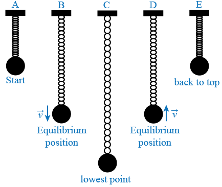
Figure 2: Five key points of a mass oscillating on a spring
Position A: The spring is compressed; the mass is above the equilibrium point at
y = A
and is about to be released.
Position B: The mass is in downward motion as it passes through the equilibrium point.
Position C: The mass is momentarily at rest at the lowest point before starting on its upward motion.
Position D: The mass is in upward motion as it passes through the equilibrium point.
Position E: The mass is momentarily at rest at the highest point before starting back down again.
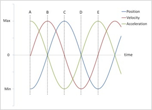
Figure 3: Position, velocity and acceleration vs. time
Mass and Spring
A mass suspended at the end of a spring will stretch the spring by some distance y. The force with which the spring pulls upward on the mass is given by Hooke's law where k is the spring constant and y is the stretch in the spring when a force F is applied to the spring. The spring constant k is a measure of the stiffness of the spring. The spring constant can be determined experimentally by allowing the mass to hang motionless on the spring and then adding additional mass and recording the additional spring stretch as shown below. In Figure 4a, the weight hanger is suspended from the end of the spring. In Figure 4b, an additional mass has been added to the hanger and the spring is now extended by an amountΔy.
This experimental set-up is also shown in the photograph of the apparatus in Figure 5.
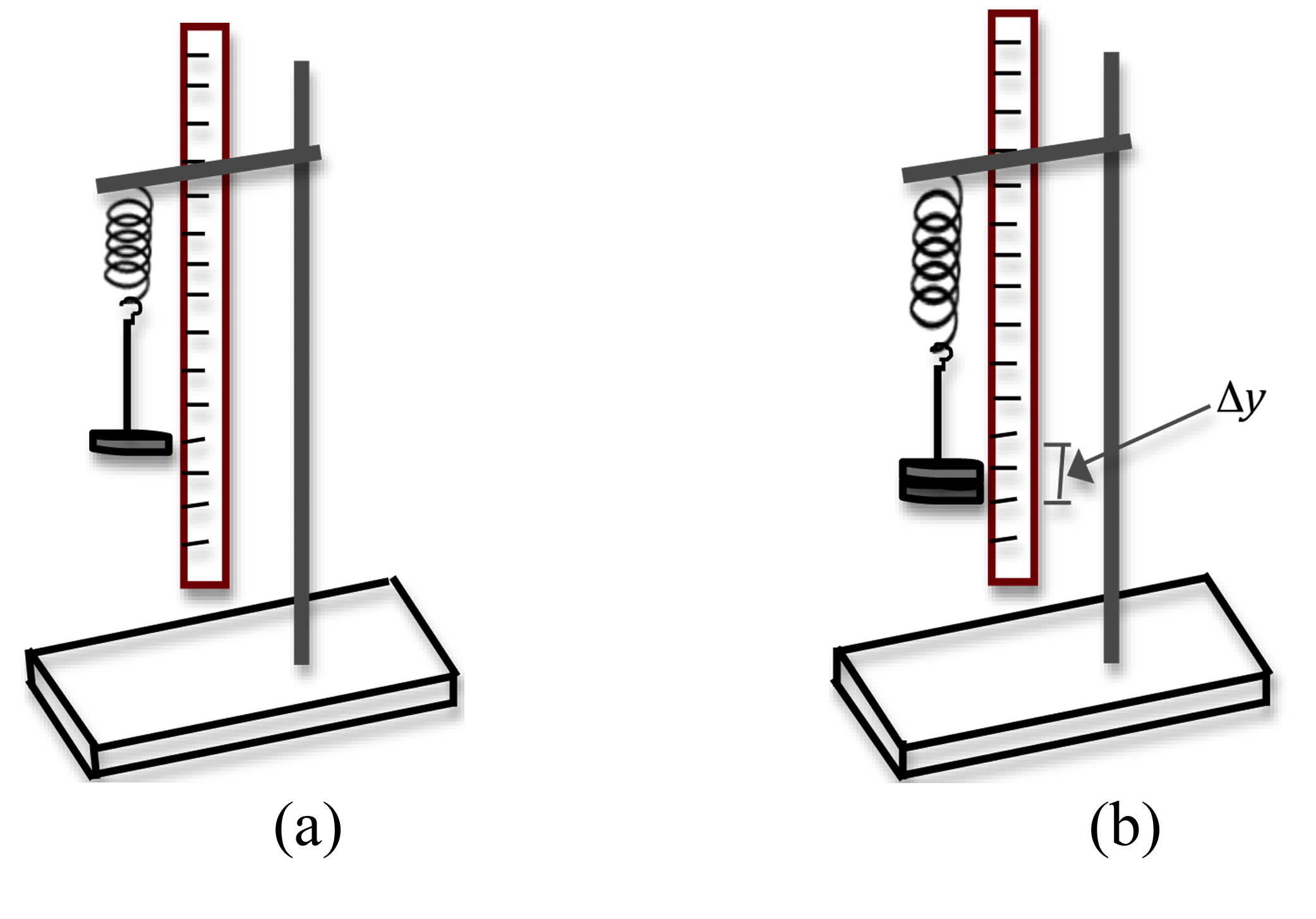
Figure 4: Set up for determining spring constant
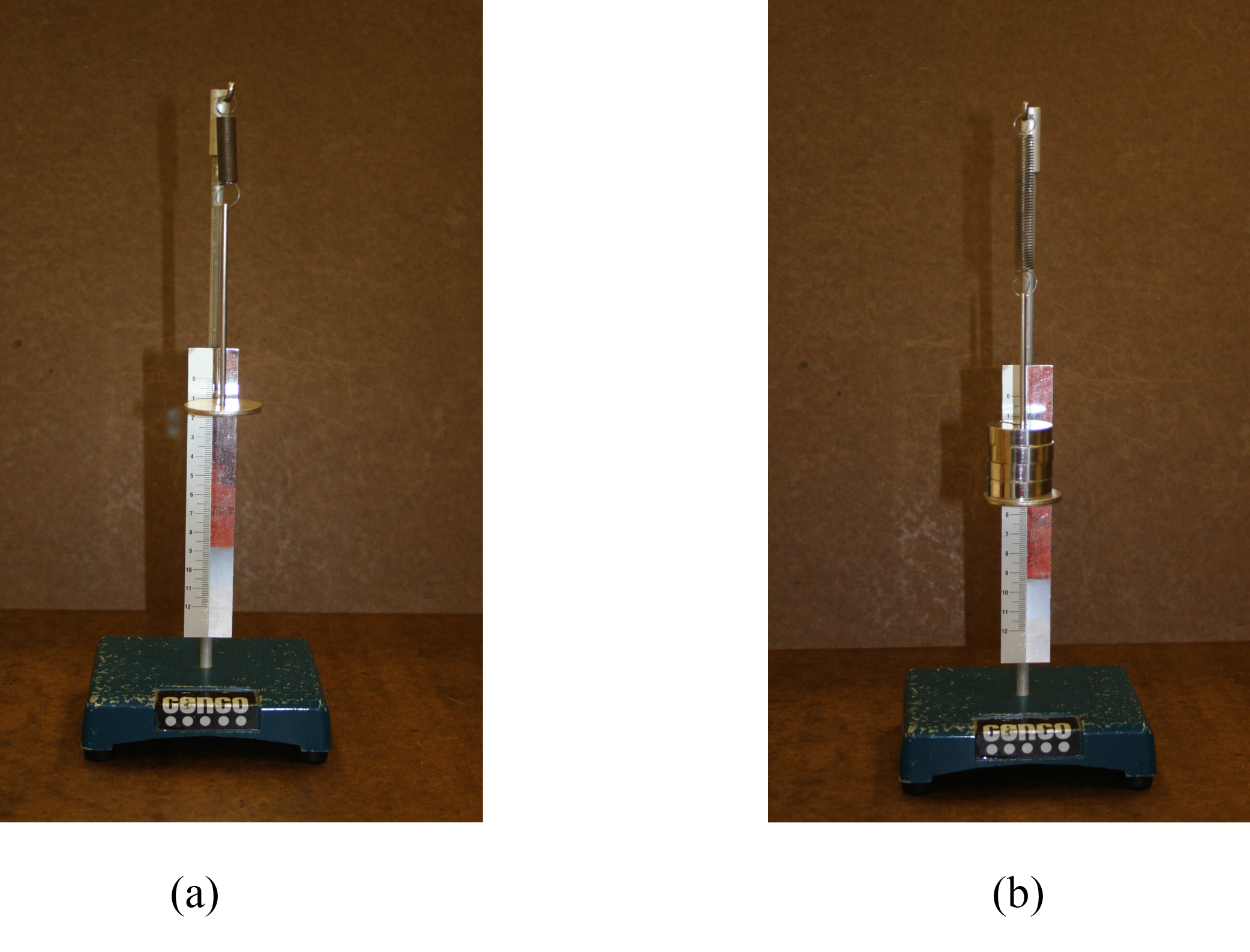
Figure 5: Photo of experimental set-up
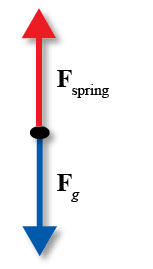
Figure 6: Free-body diagram for the spring-mass system
Δm
is the change in mass and Δy
is the change in the stretch of the spring caused by the change in mass, g is the gravitational acceleration, and k is the spring constant. Equation 7 can also be expressed as
Newton's second law applied to this system is ma = F = −ky.
Substitute from equation 5a = −4π2f2y.
for the acceleration to get
from which we get an expression for the frequency f and the period T.
Using equation 11, we can predict the period if we know the mass on the spring and the spring constant. Alternately, knowing the mass on the spring and experimentally measuring the period, we can determine the spring constant of the spring.
Notice that in equation 11, the relationship between T and m is not linear. A graph of the period versus the mass will not be a straight line. If we square both sides of equation 11, we get
Now, a graph of 
T2
versus m will be a straight line, and the spring constant can be determined from the slope.
Simple Pendulum
The other example of simple harmonic motion that you will investigate is the simple pendulum. The simple pendulum consists of a mass m, called the pendulum bob, attached to the end of a string. The length L of the simple pendulum is measured from the point of suspension of the string to the center of the bob as shown in Figure 7 below.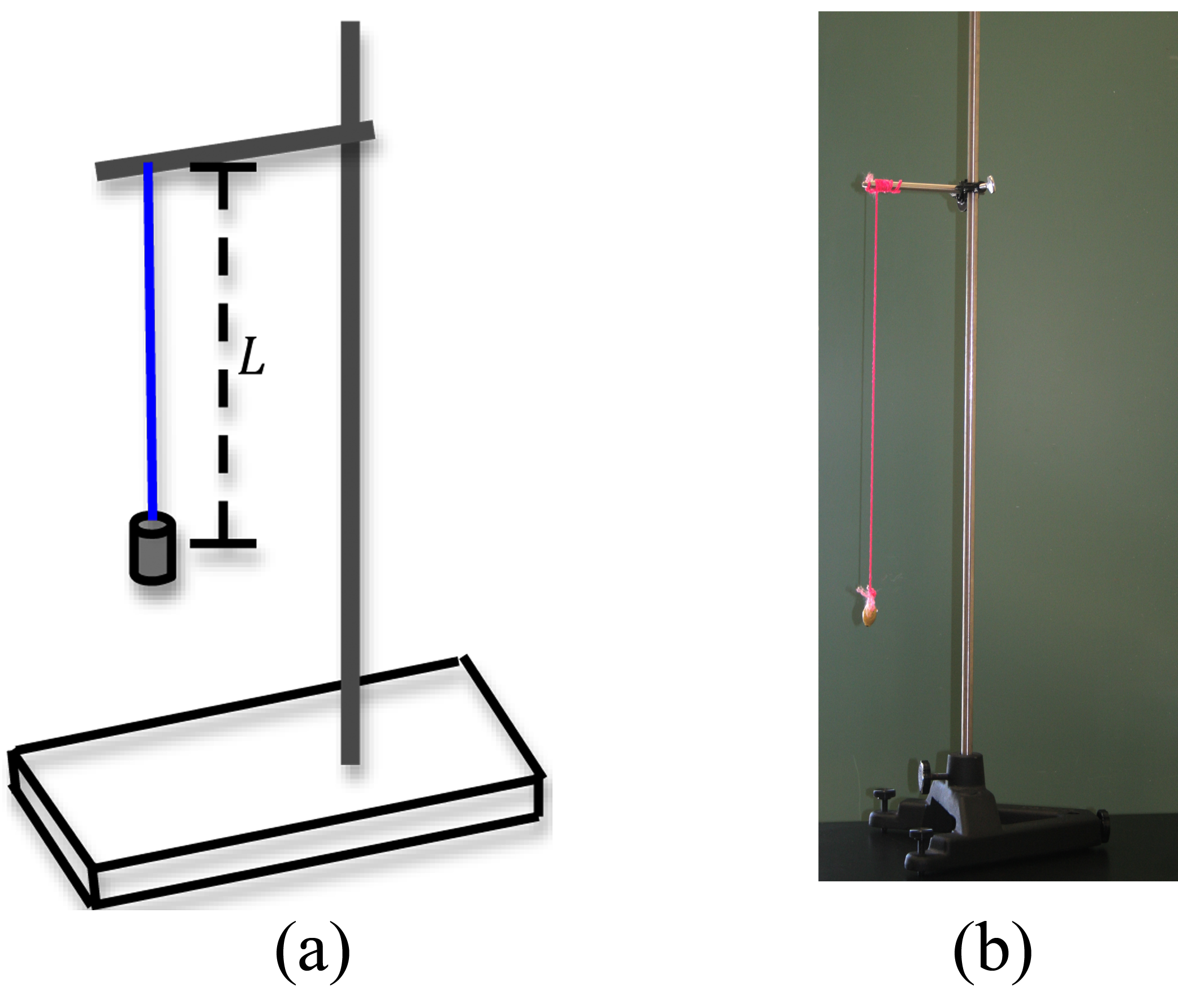
Figure 7: Experimental set-up for a simple pendulum

Figure 8: Simple pendulum
α = a/L.
From equation 13 we get
In Figure 9, the blue solid line is a plot of sin(θ) versus θ, and the straight line is a plot of θ in degrees versus θ in radians. For small angles, these two curves are almost indistinguishable. Therefore, as long as the displacement θ is small, we can use the approximation 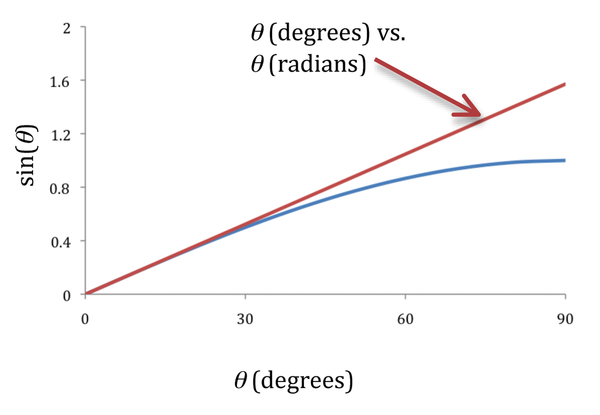
Figure 9: Graphs of sin θ versus θ
α = −
sin θ.
becomes
Equation 15 shows the (angular) acceleration to be proportional to the negative of the (angular) displacement, and therefore the motion of the bob is simple harmonic and we can apply equation 5| g |
| L |
a = −4π2f2y.
to get
Combining equation 15 and equation 16 and simplifying, we get
and
Note that the frequency and period of the simple pendulum do not depend on the mass.