
Motion with Constant Acceleration
Introduction
Newton's second law describes the acceleration of an object due to an applied net force. In this experiment you will use the ultrasonic motion detector to study the motion of a low friction cart moving on a track that is inclined with the cart accelerated by gravity.Theory
When an object is placed on a "frictionless" inclined plane, there are two forces acting on it: the force, W, due to gravity and the normal force, N, exerted on it by the plane. Since the plane is assumed to be frictionless, there is no component of this contact force parallel to the plane. If the x- and y-axes of the system are chosen to be parallel and perpendicular to the incline of the plane respectively, then the weight, mg, can be resolved into its components as shown in Figure 1.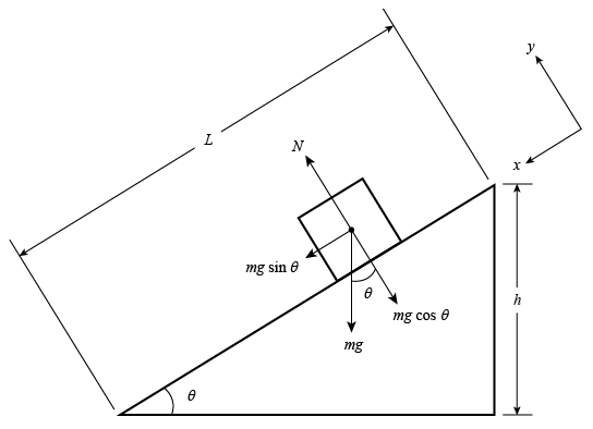
Figure 1
g =
. Thus g can be determined by measuring the quantities x, L, h, and t.
| 2xL |
| ht2 |
Objectives
The objective of this lab experiment is to make simultaneous experimental observations of the position, velocity, and acceleration of a uniformly accelerating object on an inclined plane. From these data, it will be possible to study the relationship between these three quantities, and make a measurement of the acceleration due to gravity.Apparatus
- Computer
- LabPro interface box
- Logger Pro software
- Vernier Motion Detector
- PASCO low-friction track with leveling screw
- PASCO collision cart with specially designed low-friction wheels
- 1-cm and 2-cm spacers
- Meterstick
- Triple-beam balance (on back tables)

Figure 2: Apparatus
Procedure – Session 1
Please print the worksheet for this lab. You will need this sheet to record your data.
A: Measuring the Acceleration of the Cart on an Incline
1
Find the motion detector and verify that it is connected to the DIG/SONIC: 2 port on the LabPro interface.
2
Double-click the Logger Pro icon on your computer screen. This should start up the Logger Pro program. Go to FILE, select OPEN, and find the folder called Probes and Sensors. Double-click on this and look for the Motion Detector folder. Double-click this and then select the Motion Detector file. In the Logger Pro window, you should see a Graph Window with three panes showing position, velocity, and acceleration on the vertical axes and time on the horizontal axes. (See Figure 4.)
You will use Logger Pro to collect data on the position of the "collision" cart (its distance from the motion detector) at regularly spaced instants in time as the cart moves along the low-friction track. From this set of distance-versus-time data, Logger Pro will calculate approximate values for the velocity and the acceleration at each sampled time and will plot the velocity and the acceleration of the cart as functions of time.
3
Set up the low-friction track and cart as shown in Figure 3. Place the 2-cm spacer under the foot of the track and place the motion detector in line with the track, 10–20 cm away from the end stop as shown in the figure.
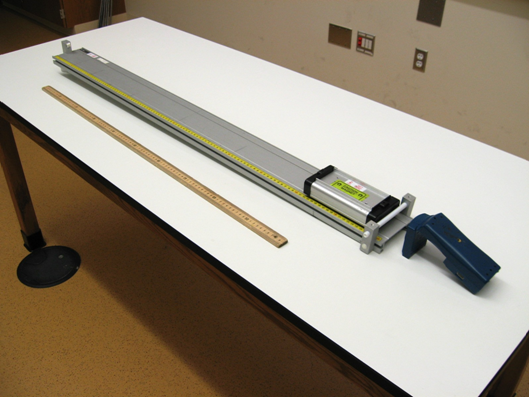
Figure 3
4
Before beginning to take data, take a moment to familiarize yourself with the Logger Pro controls. It is also helpful to see how the positioning of you and your lab partners when taking this data can influence the data being collected.
The experiment will work best if one of the partners controls the data acquisition, one launches the cart and catches the cart as it rolls toward the end stop, while the remaining partners stay back out of the range of the sonic rangers.
5
When your data looks like that in the example below, with smoothly changing position and velocity and an approximately constant acceleration, you are ready to take data. (See Figure 4 for an example of what the data should look like.) Turn on the data collection and release the cart near the top of the ramp. Catch the cart before it hits the end of the track and keep it motionless until the data collection stops (you will hear the sonic ranger stop clicking). The data collected will be used in part B. You should export this data in CSV format to the desktop in order to carry out the analysis in part B.
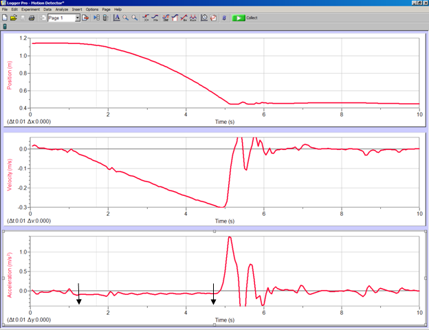
Figure 4
B: Determine the Average Acceleration Using the Acceleration Graph
1
On the desktop, open the CSV file you saved in part A using Excel. Next, with the file open, you want to make three separate graphs: the position vs. time, the velocity vs. time, and the acceleration vs. time for this data. You can do this by highlighting the data that you wish to graph and then clicking on insert scatter plot in the tool bar. Start with the acceleration vs. time graph first, since this graph will help you see which range of data in the table you will want to study more carefully. When the acceleration vs. time graph is displayed, you will want to determine the time range over which the value of the acceleration is behaving as though it is a constant. Why should we expect this behavior? The two arrows on the acceleration graph in Figure 4 point out the region of uniform acceleration for this data run. Note the beginning and end times for this interval and then replot all three of these motion graphs over this interval.
Focusing first on the acceleration vs. time graph, select eight points in this time interval to find the value of the acceleration at these eight different times and copy them to a new tab in your workbook. Note the times corresponding to the first and last data points in the set of eight data points that you use.
2
Using your data and the tools within Excel, calculate the average (mean) acceleration for these eight acceleration measurements and the standard deviation for this average.
C: Determine the Average Acceleration Using the Velocity Graph
1
Using the same data found in part A, and now using the velocity graph (not the acceleration graph), determine the average acceleration for this same time interval. The average acceleration of the cart for a given time interval is the average slope of the v(t) curve. You can get the slope of the velocity curve by adding a "trendline" to the velocity vs. time graph. Read the velocity and time at the initial and final times you used in the previous step. Determine the average acceleration by dividing the change in velocity by the change in time. The error on your velocity calculated in this way is found using the propagation of errors technique for finding (ΔV/Δt) = aave.
2
Compare this result to the one obtained from the acceleration graph. Did you expect them to agree? Discuss with your lab partners how you might account for any disagreement between the two results for the average acceleration.
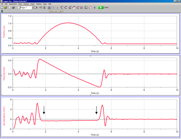
Figure 5
D: Determine g from Average Acceleration of the Cart on an Incline
1
Elevate the track using the 3-cm spacer. With the cart positioned at the lower end of the track, give the cart a gentle push so that it rolls uphill. Before beginning to collect data, take a moment to practice rolling the cart up the ramp with the data recording turned on. You will need to learn how much force you will need to launch your cart up the ramp without running to the end stop at the top of the ramp, and by looking at the data being recorded you will get a feel for how best to get the cart smoothly rolling up and down the incline. It is also helpful to see how the positioning of you and your lab partners when taking this data can influence the data being collected.
The experiment will work best if one of the partners controls the data acquisition, one launches the cart, and the remaining partners stay back out of the range of the sonic rangers.
When you are ready to take data, turn on the data recording and then launch the cart uphill so that it stops before reaching the end of the track and then rolls back down the ramp to its starting position. Catch the cart before it hits the end stop at the bottom of the track and hold the cart motionless until the sonic ranger stops clicking. You should see graphs that look similar to those shown in Figure 5.
2
Take a data run and export the data collected to the desktop as a CSV file. Next, open the file using Excel as you did in the earlier part of the experiment. Once again you will need to make three graphs of the position, velocity, and acceleration of the cart during its motion. For this analysis you want to find the time range where the cart is rolling with a uniform acceleration. In the figure above, the arrows on the graph indicate this region. Adjust the time range in your spreadsheet until they span this same time range and copy this data onto a new workbook page. Next, identify an interval of your v(t) data that is between the time at which you released the cart and the turning point—the time at which the cart momentarily stopped and changed direction. Select this range of velocities and times and make a new velocity vs. time graph for these data. Once this data is graphed, use the Excel tools to add a linear trendline to the graph. You should see a straight line passing through the portion of the v(t) curve that you selected. The slope, y-intercept, and fit parameters can be displayed on the graph by choosing this option when setting up the trendline fit. The slope, m, of the line is a direct measure of the average acceleration of the cart during the selected time interval.
3
Using the data taken in step 1, record the acceleration, a, of the cart and its standard deviation, Δa, in the "uphill."
4
Do another linear fit for a time interval between the turning point and the time at which the cart was brought to rest. Record the acceleration, a, and its standard deviation, Δa, for these "downhill" data.
5
Now repeat steps 1 and 2 for a total of three separate data trials. (You should now have a table of data with six entries—three for the "uphill" and three for the "downhill.")
6
Measure enough parameters to accurately determine the angle of the incline of the track. Record this angle and your estimate of the error in your measurement.
7
Using your measured values of acceleration from steps 3 and 4, calculate the corresponding values of g (six more entries).
8
Calculate and record the average value for the acceleration and the average value for g along with their respective standard deviations for our measurements.
9
Do your "uphill" and "downhill" measurements produce the same results? Discuss your results with your lab partners.
10
Sketch the free-body diagrams for the cart during the "uphill" and "downhill" parts of its motion to try to understand any differences between the "uphill" and "downhill" data.