
Investigating Springs (Simple Harmonic Motion)
Introduction
The purpose of this lab is to study the well-known force exerted by a spring. The force, as given by Hooke's Law, is a function of the amount the spring is stretched or compressed and therefore the constant force formulae and resulting trivial potential energy functions do not apply. The motion of an object suspended from an ideal spring, in the absence of any friction, is called Simple Harmonic Motion. This type of motion occurs in a wide variety of physical systems and is itself worth studying. You can also obtain the potential energy function for the spring force and test the Law of Conservation of Energy. Everything seems to work out exactly as expected. However, when the force of the spring is investigated as a function of the mass of the object suspended from it, there is a puzzling result.Determining the Spring Constant
When a mass, m, is suspended from a spring the extension of the spring at the equilibrium position can easily be measured. From the free body diagram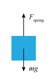
Figure 1
xeq
is the extension of the spring at equilibrium (note: a downward stretch is a negative displacement), k is called the spring constant and from the above we have
Conservation of Energy and Simple Harmonic Motion
We have seen in lecture that the spring force is a conservative force like gravity and as a result can be represented by a potential energy function where x is the displacement measured from the springs equilibrium position and the C's are arbitrary constants. Then using the Work-Energy Theorem, the total energy of a moving mass on the end of a spring in the presence of a uniform gravitational acceleration is given by If we start such a mass moving about its equilibrium position, we see that the mass will undergo a repetitive oscillation until these oscillations gradually die away and the object is once again at the equilibrium position. This motion as noted above is often described as Simple Harmonic Motion. During these oscillations, we observe that the period of the oscillations remains approximately constant despite the fact that the oscillations are gradually dying away. If we investigate this system of mass and spring further using Newton's Laws, we can write down the equations of motion for this mass undergoing these oscillations and we find the following. The details of solving this equation will be discussed in the text and lecture, however from our observation of this system undergoing these oscillations, we appreciate that the solutions must be some form of oscillatory functions like sine and cosine of ωt. If we set the origin of our coordinate system at the equilibrium position of the mass on the end of the spring when it is at rest, we can then write down the solution of this equation as where and the period of these oscillations is given by To see that this function does indeed satisfy the equations of motion, substitute it into the equation and see what results. Note, in these calculations, we have assumed that the mass of the spring is negligible, however, if we allow the spring to have a mass and do the calculus necessary to solve the modified equation of motion, we find that the period of oscillation is modified as follows where the effective mass of the spring is
meff =
.
| mspring |
| 3 |
Objectives
In this lab, you will investigate the properties of a simple mass-spring system,-
1to make static measurements of the spring constant and the dependence of the stretch of the spring from equilibrium to the force being applied to it,
-
2then to make dynamic measurements of the mass and spring system while oscillating to investigate simple harmonic motion in this system,
-
3and lastly, observe the effect of the spring mass on the period of the Simple Harmonic Motion.
Apparatus
- Electronic stop clock
- Mass holder
- Slotted mass set
- Spiral spring
- Support rod and base
- Ruler (taped to support rod)
- Balance

Figure 2
Procedure
Please print the worksheet for this lab. You will need this sheet to record your data.
Method I: Static Measurements
1
Hang the spring from the eye-bolt at the top of the support rod. Hook the mass holder onto the bottom end of the spring and if necessary add enough slotted masses to the mass holder to just separate the coils of the spring. Observe the position of the bottom of the mass holder on the ruler. Call this value y0 and record its value.
2
Now add additional mass, ΔM, to the mass hanger and let the mass hang at rest. Do this for each value of ΔM given in Table 1. Note the position, y, on the scale of the bottom of the mass holder. The change in length, Δl, of the spring in each case is y − y0.
Record your measured values of y for each ΔM in Table 1 and enter the quantity Δl = y − y0.
Note that in Table 1 ΔM is in grams and Δl is in cm. Convert your values of ΔM to kg and your Δl to meters and record in Table 2.
3
Open Excel and plot the data in Table 2, with Δl on the vertical axis and ΔM on the horizontal axis. Use Excel to find the slope of the straight line that best fits your data.
According to the equation
k(Δl) = g(ΔM),
the vertical intercept of the line should be zero. If the vertical intercept of your line is not small or if your data does not fall close to a straight line, you have made an error in measuring, recording or plotting your data. If this is the case and you and your lab partner can't find what is wrong, ask your lab TA for help.
Record the numerical value of the slope of the line in your Excel graph.
4
Using g = 9.80 m/s2
and the slope of the line, calculate k, the force constant of the spring. Since this value of k was determined using Method I, we will call it kI.
Method II: Dynamic Measurements
1
Use the balance to measure the mass of the mass holder and record your value.
2
Hang the mass holder from the lower end of the spring and place a 40 gram slotted mass on the mass holder. Enter the total mass, M, the mass of the slotted mass plus the mass of the holder, in column 2 of Table 3. In column 3 enter the total mass converted to kg.
3
Displace the mass by about 3 cm downward from the equilibrium position and release to initiate Simple Harmonic Motion. Choose a reference point (the lowest point in the motion works well) and start the stop clock as the bottom of the loaded mass hanger moves past this point.
Start counting with zero (not one) when the stop clock starts and count each time the load passes the reference point, going in the same direction.
Stop the stop clock when 10 oscillations have been completed. Enter this time as t10(1) in column 4 of Table 3. Repeat the measurement with the other lab partner starting and stopping the stop clock. Enter this time as t10(2).
4
Calculate T, the period, as T =
and enter into the table.
| t10(1) + t10(2) |
| 20 |
5
Repeat the measurements and entries into Table 3 for each value of the slotted mass on the holder that is given for the rows of the table.
6
Open Excel and plot T (in seconds) versus M (in kg). Does your data fall close to a straight line?
7
Now plot T2 (in s2) versus M (in kg).
Your data should fall close to a straight line. If it doesn't, then you have made an error in measuring, recording or plotting your data. If this is the case and you and your lab partner can't find what is wrong, ask your lab TA for help.
Use Excel to calculate the slope of the straight line that is the best fit to your data and record that value.
8
Use the slope of the line in your Excel graph to calculate the force constant of the spring. Note that the calculation doesn't require knowing the value of g, the acceleration due to gravity at your location. Since this value of k was determined using Method II, we will call it kII.
9
The force constant of the spring has been measured two different ways. The average value of the two results is kav =
.
The percentage difference in the two values is given by | kI + kII |
| 2 |
% diff =
× 100%.
Record the percentage difference for your two values of k.
If you have been careful with your measurements and if you have done the analysis correctly, the percentage difference between your two values of k should be less than 10%. If this is not the case, look over what you have done and ask your TA for help if you can't find where you went wrong.
| |kI − kII| |
| kav |
Determining the Effect of Using a Real Spring
1
Note that our original calculation of the period depended only the mass hanging on the spring, so as the mass goes to zero so should the period. Take a look at your data and observe what the y-intercept of the T2 versus M graph is for your Dynamic Measurements. (The y-intercept is the value of T2 when M = 0.) Record the value of the y-intercept.
Remember in our equations of motion for the spring and mass, we did not include the mass of the spring, assuming that it was a massless, ideal spring. However, if we allow the spring to have mass, we must add an effective mass for the spring to the mass on the end of the spring to solve these equations fully. This added spring mass alters the expression for the period as follows,
T = 2π
.
For a typical spring meff is given by  |
|
meff =
,
where mspring is the mass of the spring.
| mspring |
| 3 |
For the graph of your data for T2 versus M in your dynamic measurements, what does Excel give for the y-intercept of the straight line that best fits your data?
2
From the value of the y-intercept and the value of the force constant k from Method II, calculate meff (the effective mass of the spring).
3
Use the balance to measure the mass mspring of the spring. Calculate | mspring |
| 3 |
4
Recall that the percentage difference between two quantities is the magnitude of their difference divided by their average, converted to a percentage. Calculate the percentage difference between your results for meff and | mspring |
| 3 |
| mspring |
| 3 |