Lab 6 - Quantum States for the Visible Hydrogen Atomic Emission Spectrum
Goal and Overview
The relationship between color, wavelength, and frequency of visible light will be determined using a Spec 20 spectrometer. The visible emission spectrum of atomic hydrogen will be analyzed in a spectrometer that has been calibrated based on the visible emission spectrum of helium. Based on the hydrogen atomic emission, the principal quantum numbers (electronic energy levels) of the initial and final states for the atoms (before and after emission) will be determined. A numerical value of the Rydberg constant will also be extracted from a graphical analysis of the emission wavelengths.
Objectives and Science Skills
-
•
Explain and use the relationship between photon wavelength and energy, both qualitatively and quantitatively.
-
•
Understand and explain atomic absorption and emission in relation to allowed energy levels (states) in an atom as well as their relationship to photon wavelength and energy.
-
•
Evaluate the precision of a spectrometer by comparing measured He* emission lines to literature values.
-
•
Observe atomic H* line spectra, fit data to the Rydberg equation, and compare experimental results to theoretical values.
-
•
Analyze and discuss factors that limit the precision of the results.
Suggested Review and External Reading
-
•
data analysis and spectroscopy information; relevant textbook information on quantum theory
Background
The study of the interaction of light with matter is called spectroscopy. Spectroscopy had been a fundamental part in the development of chemical molecular theory, and it can be used for both qualitative and quantitative analysis of matter. Most modern chemistry, biology, geology, astronomy, and physics labs use some type of spectroscopy.
Wave-Particle Duality of Light and Matter
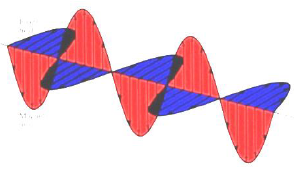
Modern wave theory says that light is composed of oscillating perpendicular electric and magnetic fields, as shown. These oscillating magnetic and electric fields are responsible for interactions of photons with the electric and magnetic properties of matter.
The speed of light, c, through a vacuum, is 2.998 × 10⁸ m/s. Light travels at different speeds through materials because of the light's interaction with the material.
-
1
The peak-to-peak distance is called the wavelength, λ.
-
2
The number of oscillations per second is the oscillation frequency, ν.
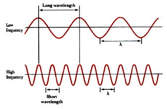
Two cases are illustrated: one wave has a wavelength three times that of the other. Wavelength and frequency are inversely proportional; as one increases, the other decreases. The two are related through the equation: λν = c. This relationship allows you to convert between wavelength and frequency.
Light can also be thought of as individual particles or packets of energy called photons. A photon has an energy proportional to its frequency, ν : Ephoton = hν = hc/λ. The proportionality constant is Planck's constant, h = 6.626 × 10⁻³⁴ J · s.
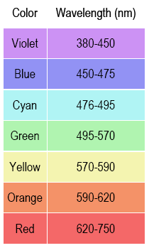
Notice that wavelength is inversely proportional to frequency. Low energy photons, like radio waves, have wavelengths of thousands of meters or more. High energy photons, like x-rays, have wavelengths of a billionth of a meter or less. Visible photons correspond to a very small part of the electromagnetic spectrum, lying between 400 (violet) and 700 (red) nanometers (1 nm = 10–9 m, or 1 m = 109 nm).
In the mid-1920s, Louis DeBroglie proposed a new notion of a wave-particle duality for matter. Wave-particle duality for light and matter quickly led to the creation and development of quantum theory.
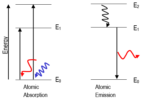
Atomic Absorption and Emission
When an atom absorbs a photon of light, its final energy, Efinal, is greater than its initial energy, Einitial; the atom experiences a
positive energy change. When an atom emits a photon, the atom's initial energy, Einitial, is greater than the final energy, Efinal; the atom
experiences a negative energy change. Absorption and emission strictly follows the law of conservation of energy: Ephoton = |ΔEatom|. The change in the atom's energy is equivalent to energy of the photon, hν.
( 1 )
ΔEatom =
ΔElevels ni → nf =
Ef −
Ei =
Ehν =
hν =
This experiment focuses on the emission of visible light from excited hydrogen atoms.
The wave description of matter explains why electrons may only exist in very specific states, or orbitals (e.g., 1s, 2s, 2p, etc.). The orbitals have very specific energies. Atoms can be "excited" to higher energy states in several ways, including strongly heating the
atom or putting it in an electric discharge or colliding it with energetic particles. The excited atoms will eventually spontaneously lose that excitation energy and "fall" to lower energy states, emitting light at wavelengths given by Eq. 1ΔEatom =
ΔElevels ni → nf =
Ef −
Ei =
Ehν =
hν =
. Atomic emission spectra are called line spectra because they appear as sets of discrete lines. This reflects the fact that atoms can only emit photons with energies corresponding to the energy difference between two discrete electronic states.
Each type of atom shows a characteristic emission spectrum, owing to its own unique orbital energies. This enables its
identification by emission spectroscopy. For example, before helium was discovered on the earth, it was found to exist in the sun because He's emission spectrum was observed in sunlight.
The hydrogen atom is the simplest atom, with the most abundant isotope consisting of one proton and one electron. The observed
emission lines of excited hydrogen atoms can be empirically fitted to a simple equation.
( 2 )
Rydberg Equation:
Ehν =
RH −
,
for ni >
nf
where nf and ni are the principal quantum numbers specifying the final and initial energy states of the H atom. RH is Rydberg's constant, and it has been shown to contain fundamental quantities like π, electron charge and mass, Planck's constant and the speed of light.
( 3 )
Rydberg's constant:
RH =
= 2.180 × 10
−18 J = 1.096776 × 10
7 m
−1
Because the H atom is relatively simple, the Schrödinger equation can be solved for the quantum states and energy levels of its electron. The math supports the experimentally-derived Rydberg equation. The allowed set of energy levels for the electron in the H atom follows the equation below.
( 4 )
En = −
, where
n is an integer = 1, 2, 3,

Note the following:
-
i
The energy of a stable H atom must obey this equation, where n, the principal quantum number, corresponds to electron orbitals. For example, n = 1 gives the energy of the 1s orbital; n = 2, the 2s and 2p orbitals; etc.
-
ii
All energy levels of H atoms are negative, which means that they are lower than the value chosen to be zero. For H atoms, the zero of energy is that of a proton and an electron separated such that the charges no longer feel each other.
-
iii
The energy level depends on 1/n2, just as the Rydberg equation shows.
When n = 1, the H atom has the lowest possible energy:
( 5a )
−RH/12 = −2.18 × 10⁻¹⁸ J; this is the ground state.
When n = 2, the H atom is in the first excited state with energy of:
( 5b )
−RH/22 = −2.18 × 10⁻¹⁸ J/4 = −5.45 × 10⁻¹⁹ J.
When n = 3, the H atom is in the second excited state with energy of:
( 5c )
−RH/32 = −2.18 × 10⁻¹⁸ J/9 = −2.42 × 10⁻¹⁹ J.
And, so on.
The wavelengths of light expected to appear in the H atomic emission spectrum can be calculated using the equation below.
( 6 )
Ehν =
RH −
=
Ef −
Ei | |
| atom |
For example, the photon energy predicted for the transition, ni = 3 to nf = 2, is below.
( 7 )
Ehν, expected =
Ef −
Ei = −
RH −
=
−5.45 × 10
−19 + 2.42 × 10
−19 J = 3.03 × 10
−19 J
Eq. 6Ehν =
RH −
=
Ef −
Ei | |
| atom |
gives the positive value, which would be appropriate for an emitted photon. You should understand that the energy change of the atom is positive for absorption (nf > ni) and is negative for emission (nf < ni).
Note the following:
-
i
Each photon wavelength (or energy) in the observed spectrum is associated with two quantum numbers (for the initial and final states).
-
ii
For emission, the initial energy is greater than the final energy, and the initial quantum number, ni, is greater than the final
quantum number, nf. The absolute value is included so that the photon energy is positive even though the energy change
of the atom is actually negative for emission.
-
iii
Evidence of quantized energy levels in matter comes from atomic emission spectra, in which photons are observed as
electrons change from one orbital to another. If electrons could have any energy, you would observe all wavelengths. However, only discrete wavelengths are emitted, and they correspond to the energy difference between two orbitals of specific energy, i.e., 1s, 2s, 2p, 3s... and so on.
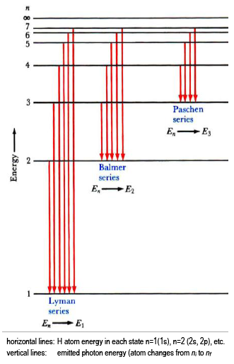
A special quality of the hydrogen atom emission spectrum is that the emitted photon energies come in separate wavelength sets, called series. In each series, all electronic transitions share a common final state (nf).
The lowest few energy levels for the H atom are shown (Eq. 4En = −
, where
n is an integer = 1, 2, 3,
), with transitions that would give rise to three series in the H emission spectrum indicated by vertical lines (Eq. 6Ehν =
RH −
=
Ef −
Ei | |
| atom |
).
The emission series shown are:
-
Lyman series, with nf = 1 (UV);
-
Balmer series, with nf = 2 (visible); and,
-
Paschen series, with nf = 3 (IR).
This lab provides you with experimental evidence that the quantum theory of matter is actually true (neat!).
You will characterize the emission of excited hydrogen atoms and verify that you are observing the Balmer series (nfinal = 2). Using your measured wavelengths (energies), you will determine the quantum numbers that fit the data and the Rydberg equation. Helium atomic emission is used to calibrate the spectrometer.
Procedure
Part 1: Visible light - wavelength vs. color
This part of the experiment is not designed to take a lot of time.
Caution:
A small Lucite rod is taped in to your Spec 20. The rod's orientation is critical, so please do not remove the tape and please do not touch the rod.
The Lucite rod transmits the light up from within so you can see the color.
1
Write the wavelengths from 400 to 760 nm at 20 nm intervals (uniformly spaced down a page in your notebook).
2
Turn the wavelength knob and note the colors you see while looking at the rod. Get a quick sense of how the colors change as you change wavelength.
3
Look carefully at the light of each wavelength at 20 nm intervals.
4
Broadly classify the color as violet, blue, green, yellow, orange, or red. Also describe the color in the most precise words that you can.
5
Record the boundary wavelength between different colors.
6
Record the wavelength where each color has its maximum intensity,
λmax.
7
Note how broad the wavelength range is for some colors and how narrow it is for others.
Part 2: Spectrometer calibration (He spectra) and usage (H spectra)
Caution:
Do not touch the high voltage discharge tubes or power supply connections.
Helium gas, He, and hydrogen gas, H2, are sealed in glass discharge tubes. These tubes can be connected to a high voltage source. The high voltage across the tube of gas creates a discharge in the gas. When a spark passes through the gas, its energy is raised greatly. These lamps are like fluorescent tubes or neon lights. In the case of He, the atoms are excited and give off radiation (some visible) as they fall back to lower energy levels. You will study this radiation in Part 2b. In the H2 tube, some H2 molecules are broken into H atoms, and many of these are in excited states. The excited H* atoms emit photons as they transition to lower energy states. Some of these photons lie at visible wavelengths. You will study this radiation in Part 2c. Excited atoms give rise to line spectra. The emission spectrum of excited H2 molecules would contain 'bands' due to the allowed vibrational levels within each electronic level.
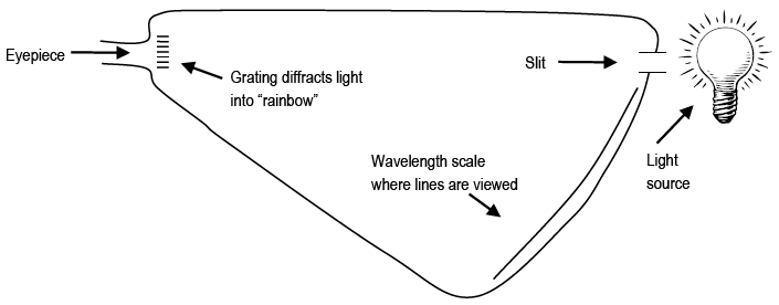
Light enters a slit in the spectrometer and is dispersed (spread out in the way a prism does). The spectrometer has an eyepiece through which you see the colored spectral lines superimposed on a wavelength scale (e.g., 6.60 × 10⁻⁵ cm or 660 nm). When observing the emission lines, it is important to be consistent in how you position your head and where you hold your eye. The position
of the lines on the scale will appear to move if you move your line of sight through the eyepiece.
Part 2a: Handheld Spectrometers (if available)
1
Using a handheld spectrometer, point the slit at the fluorescent lights in the ceiling. Note the spectral lines in the eyepiece. The bright blue and green lines you see are mercury atom emission.
2
Adjust the side shutter on the spectrometer to let more or less light in to illuminate the wavelength scale. The more light you get on the scale, the harder it is to see your spectral lines.
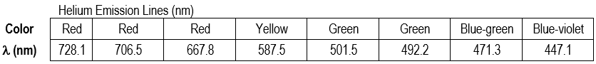
Part 2b: Helium Emission Lines
The types of spectrometers we use are not highly precise instruments, but their accuracy should be relatively good.
You will use the emission wavelengths of excited helium atoms to assess the accuracy of the instrument.
1
Point the table-top spectrometer towards the He discharge tube and position the slit so that you observe colored lines on the scale. Write down the wavelength and color of each observed spectral line. You may not see all of the lines. Some are too close to each other to distinguish individual lines; the lowest- and highest-wavelength lines can also be hard to observe.
2
Even though the theoretical wavelength values are to four significant figures, the difficulty in reading the spectrometer's scale limits the precision to which you can read wavelength. An uncertainty of ±10 nm around the wavelength value you report is typical.
Note: Since you can only estimate the position of the emission lines within ±10 nm precision, your uncertainty is ±10 nm, and your reported wavelengths for the He and H emission should be reported to the ±10 nm (e.g., 660 nm, not 656 nm).
3
Compare theoretical wavelength values to your experimental wavelengths. Calculate the percent error in each that you observed to two significant figures. How accurate is your spectrometer?
Part 2c: Hydrogen Atomic Emission
1
The lines of the hydrogen atomic emission spectrum in the visible are known to be at
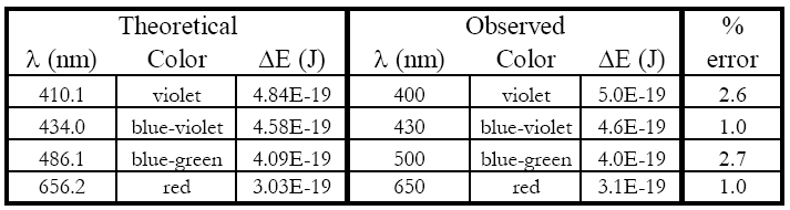
410.1, 434.0, 486.1, and 656.2 nm.
2
View the hydrogen gas tube with the spectrometer that you used in part 2b. Note the multi-colored bands due to excited H
2* molecules. These are not present in the He emission because helium exists naturally as atoms.
3
Position your head so that the bright blue-green emission line shows on the same about 490 nm. Do not move your head from this position. Write down the wavelength (to ±10 nm) and the color of each observed H* emission line. You should have 3 or 4 values.
4
Calculate the energy of each emitted photon to two significant figures in Joules using
Eq. 1ΔEatom =
ΔElevels ni → nf =
Ef −
Ei =
Ehν =
hν =
The calculated energy equals the change in atom's energy, Efinal − Einitial = ΔEatom.
The atom's energy change is negative even though photon energy is usually given as positive. The emission wavelengths that are in the visible range for the H atom are known to be those of the Balmer series (nf = 2).
Are your values similar?
Note
nf = 2;
ni = 3, 4, 5, and (maybe) 6.
6
Calculate the percent error in each experimental energy relative to each known literature value (to two significant figures).
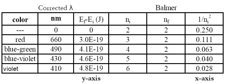
A set of example data is shown. Calculations were performed in Excel®, so scientific notation appears as #E# instead of # × 10
#. You must use your own values.
Hopefully, you will see only a small percent error. This experiment supports the quantum mechanical treatment of the atom (and you saw it in lab).
Your data also allow you to determine an experimental value for the Rydberg constant—how does yours compare to the true value?
7
To determine your experimental value of the Rydberg constant,
RH, you need to rearrange the Rydberg equation into the form of a
straight line:
( 8 )
| Ehν = RH − | ⇒ | ΔEatom | = | −RH | | + | |
| | y | = | m | x | + | b |
where
slope = −
RH,
y-intercept =
,
x values:
, and
y values:
Ehν.
8
Plot
Ehν for each emission line vs. 1/
ni2 (recall
nf = 2 for the Balmer series). The points should lie on a straight line.
-
a
You should have 3 or 4 data points for the graph, one for each photon energy and its associated initial state, ni.
-
b
The lowest energy photon (at the red end of the spectrum) corresponds to the lowest energy transition. For the Balmer series this would be ni = 3 → nf = 2. The energies increase as the wavelengths decrease.
-
c
Draw a best-fit line through the points on your graph.
-
d
Determine the slope of the best-fit line to three significant figures. Pick two points on the line, one near the top and one near the bottom. The slope is ΔEhν over Δ(1/ni2) values (this is rise over run, or Δy/Δx).
-
e
Confirm you have selected the correct series (value for nf) by checking three values from your graph.
-
i
The slope of your best-fit line should be approximately –RH. Find the percent error relative to the true value
(RH = 2.18 × 10⁻¹⁸ J).
-
ii
The y-intercept should be RH/nf2 (2.18 × 10⁻¹⁸ J/22); find your value to three significant figures.
-
iii
The x-intercept (the point where the line crosses the x-axis) should be the point at which ΔE is zero and 1/ni2 = 1/nf2 = 1/22.
Three significant figures are fine for this value.
For the Balmer series, nf = 2. The line on which your data points lie should have a y-intercept = RH/4 and a x-intercept of 1/4 (1/nf2 = 0.250).
The slope should be negative.
An example plot is shown using the data from above.
-
-
-
| Experimental: | | slope (RH, exp) | ~2 × 10⁻¹⁸ J | | x−intercept | ~0.245 |
| Literature: | | RH, lit | 2.18 × 10⁻¹⁸ J | | 1/nf2Balmer | 0.250 = 1/22 |
NOTE: YOU MUST USE YOUR OWN EXPERIMENTAL DATA. IT WILL NOT BE EXACTLY THE SAME AS THE EXAMPLES GIVEN.
Reporting Results
Complete your lab summary or write a report (as instructed).
Abstract
Results
-
Wavelength versus color observations
-
He emission calibration data and plot
-
H emission wavelength (measured and corrected) data, colors, and error
-
Calculated value table – theoretical ΔE, measured ΔE, etc. (see example table)
-
Rydberg plot, experimental RH and error (relative to literature value)
Sample Calculations
-
Photon energy
-
Energy level calculation and ΔE calculation
-
Rydberg slope and error
Discussion
-
What you did, how you did it, and what you determined
-
Spec 20 color to wavelength correlation
-
Spectrometer Calibration – purpose, etc.
-
H atom emission spectra and the Rydberg plot
-
Experimental Rydberg constant?
-
What is nf for observed emission? Which series is this?
-
What is ni for each observed photon?
-
What else can you conclude from this study?
Review