
Appendix A: Basic Concepts of Error Analysis and Error Propagation
Back to TopSignificant Figures
The laboratory usually involves measurements of several physical quantities such as length, mass, time, voltage and current. The values of these quantities should be presented in terms of Significant Figures.
For example, the location of the arrow is to be determined in the figure below.
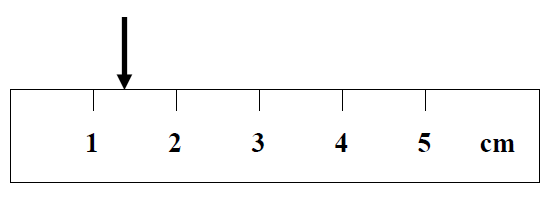
It is obvious that the location is between 1 cm and 2 cm. The correct way to express this location is to make one more estimate based on your intuition. That is, in this case, a reading of 1.3 cm is estimated. This measurement is said to contain two significant figures. Note that there should only be one estimated place in any measurement. If data are to contain, say, three significant figures, two must be known, and the third estimated. Do not try to locate the position of the arrow in fig. 1 as 1.351 cm.
It is obvious that the location is between 1 cm and 2 cm. The correct way to express this location is to make one more estimate based on your intuition. That is, in this case, a reading of 1.3 cm is estimated. This measurement is said to contain two significant figures. Note that there should only be one estimated place in any measurement. If data are to contain, say, three significant figures, two must be known, and the third estimated. Do not try to locate the position of the arrow in fig. 1 as 1.351 cm.
-
aSpecify the measured value to the same accuracy as the error. For example, we report that a physical quantity isx = 3.45 ± 0.05,not3.4 ± 0.05and not3.452 ± 0.05.
-
bWhen adding or subtracting numbers, the answer is only good to the least accurate number present. For example,50.3 + 2.555 = 53.9and not 52.855.
-
cWhen multiplying or dividing, keep the same number of significant figures as the factor with the fewest number of significant figures. For example,5.0 · 1.2345 = 6.2and not 6.1725.
Types of Errors
Every measurement has its error. In general, there are three types of errors that will be explained below.Random Errors
This type of error is usually referred to as a statistical error. This class of error is produced by unpredictable or unknown variations in the measuring process. It always exists even though one does the experiment as carefully as is humanly possible. One example of these uncontrollable variations is an observer's inability to estimate the last significant digit for a given measurement the same way every time.Systematic Errors
This class of error is commonly caused by a flaw in the experimental apparatus. They tend to produce values either consistently above the true value, or consistently below the true value. One example of such a flaw is a bad calibration in the instrumentation.Personal Errors
This class of error is also called "mistakes." It is fundamentally different from either the systematic or random errors stated above, and can be completely eliminated if the experimenter is careful enough. One example of this type of error is to misread the scale of an instrument.Mean and Statistical Deviation
Let's assume that both the systematic and personal errors can be eliminated by careful experimental procedures, then we can conclude that the experimental errors are governed by random statistical errors. If there are a total number of N measurements made of some physical quantity, say, x, and the i-th value is denoted by xi, the statistical theory says that the "mean" of the above N measurements is the best approximation to the true value; i.e., the meanx
is given by
where Σ means summation.
In cases where the uncertainty in the measurements is due to random errors, the measure of the uncertainty (random error) in the mean value will be the standard deviation of the mean (standard error), which is the precision of the mean,
where σx is a standard deviation that can be calculated using the following equation.
The statistical theory states that approximately 68% of all the repeated measurements should fall within a range of plus or minus σ from the mean, and about 95% of all the repeated measurements should fall within a range of 2σ around the mean. In other words, if one of your measurements is 2σ or farther from the mean, it is very likely that it is due to either systematic or personal error.


Reporting of Results
Typically, in the laboratory, one will be asked to make a number of repeated measurements on a given physical quantity, say x. The measured value is customarily expressed in the laboratory report as wherex
is the mean and σx
is the standard deviation of the mean.
Propagation of Errors
The mean value of the physical quantity, as well as the standard deviation of the mean, can be evaluated after a relatively large number of independent similar measurements have been carried out. These calculated quantities in many cases serve as a basis for the calculation of other physical quantities of interest. For instance, in the laboratory, speed is determined indirectly by the division of the distance traveled and the time taken to travel that distance. In such situations, the uncertainties associated with the directly measured quantities affect the uncertainty in the quantity that is derived by calculations from those quantities. To estimate the uncertainty (error; standard/random error or standard deviation of the mean) in the final result, the error needs to be propagated. In evaluating the speed, these errors on distance and time will pass on to the speed. The rules of error propagation for the first approximation are the following, where f (function) is the derived physics quantity, Δf is an uncertainty in the derived quantity,x
and y
(variables) are the mean values of the quantities that are being measured, and Δx and Δy are uncertainties (standard deviation of the mean) in these mean values.
Rule 1: Addition/Subtraction: f(x, y) = x + y or f(x, y) = x − y
For example,(3.0 ± 0.1) + (4.0 ± 0.2) = 7.0 ± 0.3,
and (5.0 ± 0.1) − (1.0 ± 0.3) = 4.0 ± 0.4.
Rule 2: Pure Product or Division Function: f(x, y) = xy or f(x, y) =
For example,| x |
| y |
(1.0 ± 0.1) · (3.0 ± 0.3) = (1.0 ± 10%) · (3.0 ± 10%) = 3.0 ± 20% = 3.0 ± 0.6,
and | (3.0 ± 0.3) |
| (1.0 ± 0.1) |
| (3.0 ± 10%) |
| (1.0 ± 10%) |
f(x, y) = xm
For example, (3.0 ± 0.3)2 = (3.0 ± 10%)2 = 9.0 ± 2 · 10% = 9.0 ± 20% = 9.0 ± 1.8.
Another way to think about this is to multiply the power (k) by the percentage error of x to obtain the error associated with z.
Rule 4: Coefficients: f(x, y) = Cx,
where C is a constant.
For example, 2(3.0 ± 0.3) = 6.0 ± 0.6.
Rule 5: Coefficients and Multiple Powers or Exponentials: f(x, y) = Cxm yn,
where C is a constant.
