Projectile Motion

Objectives

•
to test the validity of the kinematics model for simple projectile motion
•
to test whether the horizontal range is directly proportional to the time of flight
•
to test whether the height is a quadratic function of time of flight
•
to test whether the slope of the x vs. t graph is horizontal velocity

Equipment

inclined plane, guided track, Science Workshop interface, photogates, time-of-flight accessory, lab jack, ball, metric ruler, plumb bob, masking tape

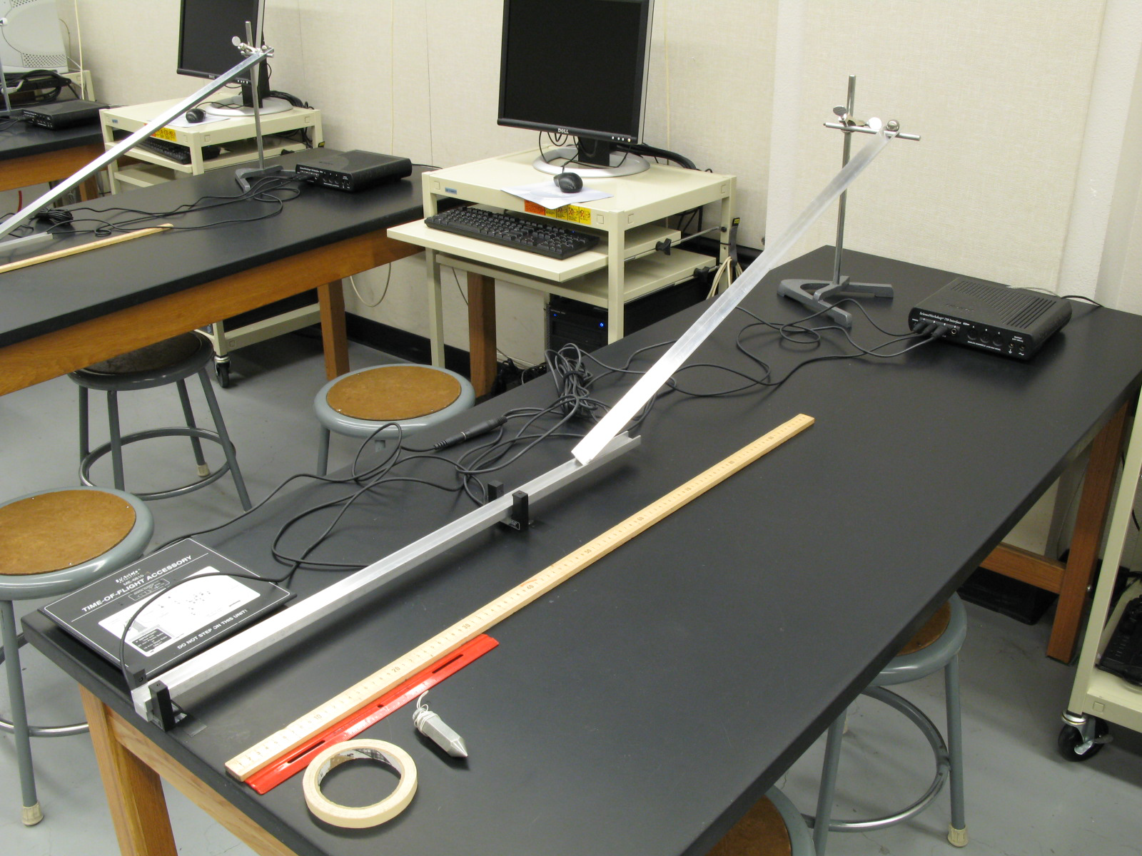
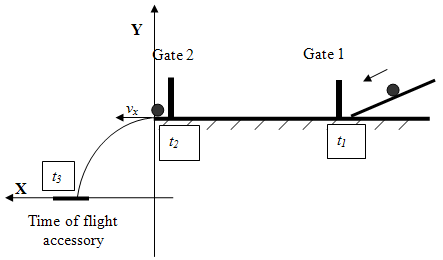
Figure 1

Figure 2: The experimental setup for the Projectile Motion lab

Introduction and Theory

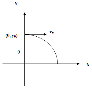
Consider the projectile motion of a ball as shown in Fig. 3. At t = 0, the ball is released at the position specified by coordinates (0, y₀) with horizontal velocity v_x. The object moves with constant velocity in the horizontal direction. The horizontal range of its motion can be found with the equation of motion used to describe constant velocity motion.

( 1 )

x = v_xt

Figure 3: The system of coordinates for the projectile's motion

Because of the influence of a constant gravitational acceleration in the Y-direction, vertical (y) components of its motion are governed by the equations used to describe a freely falling object,

( 2 )

y = y₀ + v_0yt +

g_yt²

( 3 )

v = v_0y + g_yt,

where g_y = –9.81 m/s² is the gravitational acceleration. The vertical and horizontal components of projectile motion are independent from each other. The set of equations (1), (2), & (3) describes a kinematics model for projectile motion launched horizontally. An object launched horizontally has zero initial velocity in the vertical direction (v_0y = 0). Thus, equations (2) and (3) can be simplified.

( 4 )

y = y₀ +

g_yt²

( 5 )

v_y = g_yt

There are two important facts to be noticed: (1) the distance the ball travels in the X-direction is directly proportional to the time of flight, which is due to the fact that there is no force acting upon the ball in that direction, and (2) the distance the ball travels in the Y-direction is proportional to the square of the time of flight, with the proportionality constant equal to one half of the gravitational acceleration. These relationships will be tested in the lab experiment. Additional information on kinematics in two dimensions can be found in your textbook.

Video

View the video below prior to beginning your lab.

Procedure

Please print the worksheet for this lab. Answer all the questions on the Lab Worksheet prior to submitting the Inlab in WebAssign.

Checkpoint:
Be sure to have your TA sign your lab worksheet, printed Inlab, and all printed graphs after each part is completed. Be sure the data can be seen on the graphs.

The experimental setup is depicted in Figs. 1

x = v_xt

and 2

y = y₀ + v_0yt +

g_yt²

Caution:
When taking measurements with the time-of-flight accessory, keep it in place by hand; otherwise, it will move on impact with the ball.

Mark on the inclined, v-shaped track the release position of the ball using the masking tape. It will stay the same for all the runs in this experiment.

Figure 4

Hang the plumb bob from the launch point straight down to the floor and mark that point on the floor with the masking tape. It will be the origin point. Fasten the measuring tape to the floor from the origin in the direction of the projectile motion. The tape will be used to measure the first part of the horizontal range—the distance from the launch point to the edge of the lab jack. Be sure that zero on the tape is lined up with the origin.

Place the ball at the launching point. Measure and record the height (h) from the bottom of the ball to the origin point marked on the floor. Record this height on your lab worksheet.

Bring the lab jack to the lowest height setting. Create a column in GA to record the height of the lab jack (h₁) from the floor. Create a calculated column to find the height of flight, which will equal the difference between h and h₁.

From the marked position on the v-track, launch the ball a couple of times to estimate the landing position of the projectile. Place the lab jack at the landing point. Attach the time-of-flight accessory to the metal plate on the lab jack using the double-sided tape.

Caution:
The time-of-flight accessory is a very delicate device—handle it with care.

Fold a piece of plain paper in half from the portrait orientation ("hamburger style") and place the black side of the carbon paper face down onto the top of the folded plain paper.

Open the preset experiment file: Desktop/pirt inst labs/PHY 113/PreSet Up Labs/Projectile motion. After the ball is launched, Data Studio will record the data automatically. Timer 1-2 (t₁₂) in Column 1 is the time it takes the ball to roll between photogate 1 to photogate 2. Timer 2-3 (t₂₃) in Column 2 is the time of flight. Photogate 2 registers the ball right before it is launched into projectile motion, and the time-of-flight accessory registers the time the ball lands. Column 3—Velocity in Gate— is a launched velocity, or, in other words, the initial horizontal velocity (v_x) of the projectile object.

Caution:
Be sure to hold the lab jack and the time-of-flight accessory in place to prevent its movement during the impact. The lab jack will have to stay in one place until all measurements for one trial are completed.

Figure 5

Set the ball at the release point. Use a flat side of the ruler as a launching device. Press the Start button. Let the ball roll and land on the time-of-flight accessory. Without stopping the recording, bring the ball back to the same release point and repeat the measurements four more times. Each time the ball passes through the photogates and hits the time-of-flight plate, a new row of data is added to the table. After all five runs are completed, to finish collecting one data set, press Stop.

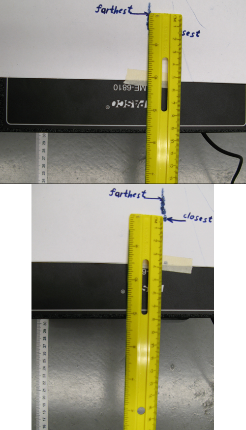
Use the cluster of positions recorded on the paper placed on the time-of-flight accessory to get the experimental value of the horizontal range (Fig. 6). Measure the distance from the launch point to the closest point of impact (X_min). Measure the distance from the launch point to the farthest point of impact (X_max). To measure the experimental horizontal range from the edge of the time-of-flight accessory to the closest and farthest points of impact, use the 30-cm ruler. Add this distance to the distance from the launch point to the lab jack measured with the measuring tape fastened to the floor. Also refer to the comments under Fig. 6. Create a column in GA to enter the values of X_min and X_max. Create a calculated column to find the experimental range traveled by the projectile ball.

Figure 6

The top image is (9.4 + 30.5) cm for the farthest point. The bottom image is (7.9 + 30.5) cm for the closest point.

In GA, create a column to enter the mean value of time of flight (t₂₃); it is provided in the second column "Timer 2-3." Create a calculated column to find t_23corr.

After the data is entered, check that the horizontal range, height of flight, and corrected time of flight are calculated automatically.

Change the height of the lab jack by at least 5 cm. Repeat steps 8–11. After all data is collected for this trial, repeat steps 8–11 of the experiment two more times with different heights. Be sure the height of the lab jack is changed for every new set of runs by at least 5 cm. You should have data for a total of 4 trials. Analyze the relationships between the quantities with the graphs.

After all data is collected, make two graphs in GA: X vs. t_23corr and height of flight vs. (t_23corr)². Apply "Linear Fit" to the graphs. Enter the slopes and their uncertainties in the Inlab on WebAssign for further calculations and analysis.

Take a screenshot of the graphs to upload a file with the graphs on WebAssign.

Complete Part 2 of the experiment following the directions provided in the Inlab.

Equations

( 6 )

h = H₀ − h_i, where i = 1...4

( 7 )

Δt_theo =

t_theo × Δy

y_exp

( 8 )

t_23corr = t₂₃ −

V_mean

d = 22 mm – the ball's diameter

( 9 )

Δt_23corr

δt₂₃

− standard deviation of the mean of Δt_23corr

( 10 )

x _theo = V_mean × t_23corr

( 11 )

Δx _theo = t_23corr ×

δ_v

+ v ×

δ_t23

( 12 )

x _exp =

x_min + x_max

( 13 )

Δx_exp

x_max − x_min

( 14 )

Δy_theo = gt_23corr × Δt_23corr