Hooke's Law

Objective

•
to test Hooke's Law by measuring the spring constants of different springs and spring systems
•
to test whether all elastic objects obey Hooke's Law

Equipment

two nearly identical springs, long rubber band, support stand with a meter stick, 50-g mass hanger, set of masses from 100 g up to 600 g, balance scale, Science Workshop Interface with force sensor and rotational motion detector used as a linear sensor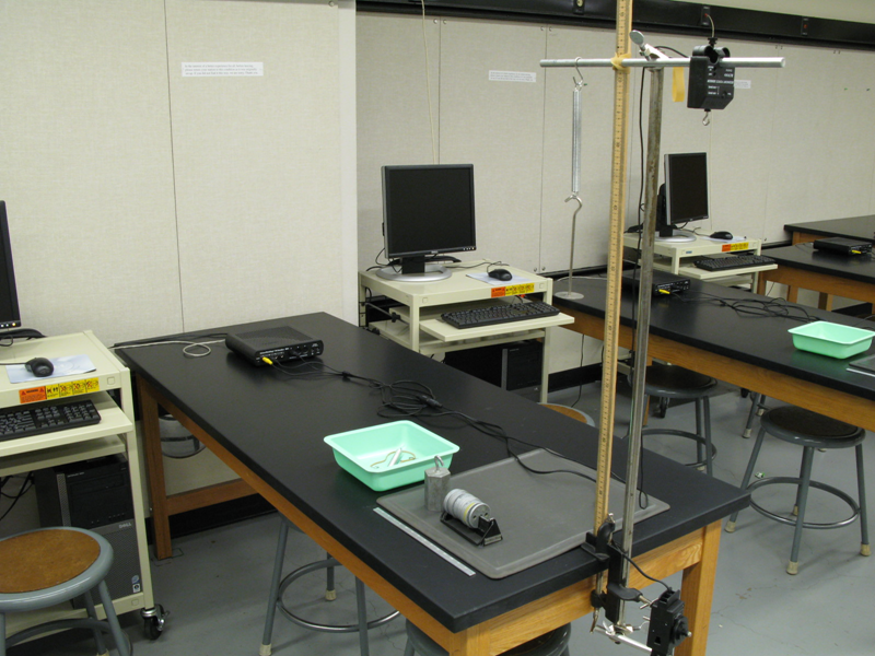

Figure 1

Introduction and Theory

Hooke's Law

Elastic force occurs in the spring when the spring is being stretched/compressed or deformed (Δx) by the external force. Elastic force acts in the opposite direction of the external force. It tries to bring the deformed end of the spring to the original (equilibrium) position. See Fig. 2.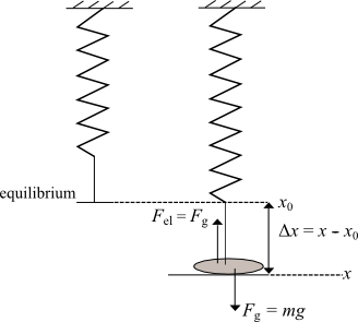

Figure 2

If the stretch is relatively small, the magnitude of the elastic force is directly proportional to the stretch Δx according to Hooke's Law:

( 1 )

F_el = −kΔx,

where k is a constant, usually called the spring constant, and Δx is a stretch (the difference between the new x and the equilibrium position). The minus sign in front of the spring constant in equation 1 indicates that the elastic force and stretch act in the opposite direction.

Procedure

Please print the worksheet for this lab. Answer all the questions on the Lab Worksheet prior to submitting the Inlab in WebAssign.

Checkpoint:
Be sure to have your TA sign your lab worksheet, printed Inlab, and all printed graphs after each part is completed. Be sure the data can be seen on the graphs.

Part 1: Measurement of a Spring Constant

The purpose of this part of the laboratory activity is to find the spring constant of the spring. The spring constant is a coefficient of proportionality between elastic force and displacement, according to Hooke's Law (equation 1

F_el = −kΔx,

). Method 1

Complete the Part 1 "Prediction" exercise on the lab worksheet before you begin the experiment.

Hang a spring from the support, add a weight hanger, and place a 200-g mass on it. This will be the equilibrium position of the system. Measure the initial equilibrium position of the hanging weight with the meter stick and record it in the Inlab.

Add masses in steps of 100 g up to 600 g and measure each corresponding position for each newly added mass. Then remove the masses in steps of 100 g and measure each position again. This will help to better identify the uncertainty.

In GA, create a table to record the experimental data of mass and position when the spring is stretched and then compressed.

Create a new calculated column to find the elastic force (DATA → NEW CALCULATED COLUMN → equation: F = variables "m"*g, where m is in kg).

Create a new calculated column for displacement (DATA → NEW CALCULATED COLUMN → equation = variables "position" – initial equilibrium position).

Make a plot of force vs. displacement. Apply "Linear Fit" to the force vs. displacement graph. Answer the questions on the lab worksheet related to the shape of the graph.

In the Inlab, record the slope of the graph and its uncertainty to find the spring constant and its error.

Take a screenshot of your graph. Be sure all data in the graph area is visible. Upload a file with the graph in the Inlab for Part 1.

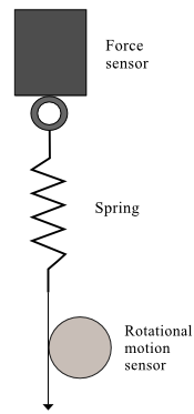
Method 2 The apparatus setup shown in Fig. 3 will be used to find the spring constant for spring 2.

Figure 3: Apparatus setup for the Hooke's Law experiment

Open the preset experiment file: Desktop/pirt inst labs/PHY 113/PreSet Up Labs/Springs.

Before taking the actual data, calibrate the force sensor. Click the Setup button in the toolbar. Then click on the force sensor icon and press the Calibrate Sensors button. This brings up the calibration panel shown in Fig. 4.

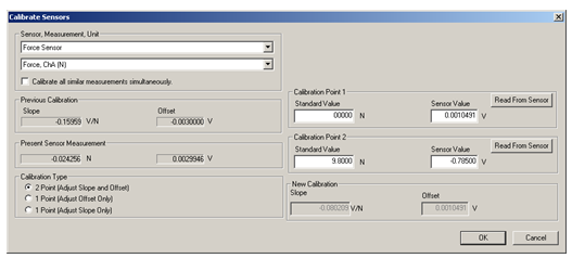
Figure 4: Calibration of force sensor in Data Studio

The "2 Point" option should be selected as the "Calibration Type." With no load on the force sensor, enter 0 in the "Calibration Point 1" standard value window. Push the Tare button on the force sensor. This action adjusts the force sensor reading to zero. Press the Read From Sensor button. Next, hang the 1-kg hooked mass on the sensor and type 9.8 in the "Calibration Point 2" standard value window. Click the Read From Sensor button. Click OK to save this calibration. Close the "Calibrate Sensors" and "Setup" windows. Now you are ready to take the actual measurements of the spring constants. (Note: If a standard mass of different value is provided, calculate "Calibration Point 2" by a product of mass and gravity acceleration.)

Replace the 1-kg weight with the spring. Attach a piece of string to it. Wrap the string around the large pulley of the rotational motion detector in a counterclockwise direction as depicted in Fig. 3. The rotational motion detector has been calibrated to read the linear distance.

Press the Start button to initiate the data acquisition. Carefully pull on the string, watching the force display window. Start releasing the string back to the original position when the force reaches 10 N.

Apply "Linear Fit" to the good part of your recording (see Fig. 5), which presents an elastic force vs. displacement graph. In the Inlab, record the value of the spring constant based on the slope of the graph.

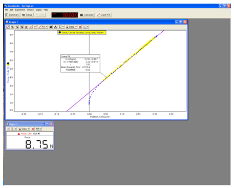
Figure 5: A sample experiment file in Data Studio

Take a screenshot of your graph. Be sure all data in the graph area is visible. Upload this graph in the Inlab for Part 1.

Part 2: Springs in Series and Parallel

Use two springs to make a system of springs in series. Repeat steps 13 and 14 from Part 1. Be sure to take a screenshot of all graphs to upload in the Inlab for Part 2.

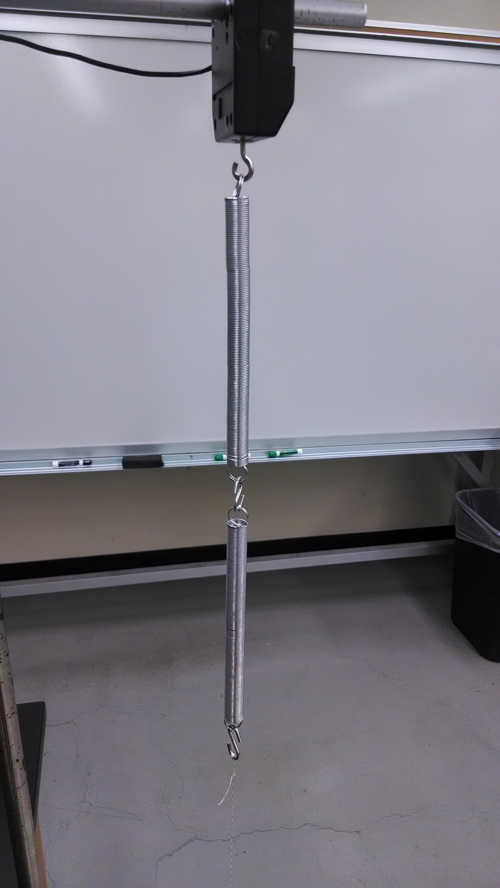
Figure 6: System of springs in series

Use two springs to make a system of springs in parallel. Repeat the steps 13 and 14 from Part 1. Be sure to take a screenshot of all graphs to upload in the Inlab for Part 2.

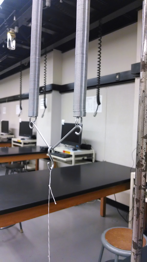
Figure 7: System of springs in parallel

Part 3: Investigation of Nonlinear Springy Object

In the experimental setup from Fig. 3, replace the spring with the long rubber band.

Repeat step 13 from Part 1 above. Record force vs. position for both down (increasing force) and up (decreasing force) strokes.

Use this data to answer the questions on the lab worksheet.