Motion In Two and Three Dimensions

CHAPTER 4

4-1	Position and Displacement

After reading this module, you should be able to …


4.01	Draw two-dimensional and three-dimensional position vectors for a particle, indicating the components along the axes of a coordinate system.

4.02	On a coordinate system, determine the direction and magnitude of a particle's position vector from its components, and vice versa.

4.03	Apply the relationship between a particle's displacement vector and its initial and final position vectors.

•

The location of a particle relative to the origin of a coordinate system is given by a position vector

, which in unit-vector notation is

Here

, and

are the vector components of position vector

, and x, y, and z are its scalar components (as well as the coordinates of the particle).

•

A position vector is described either by a magnitude and one or two angles for orientation, or by its vector or scalar components.

•

If a particle moves so that its position vector changes from

, the particle's displacement

The displacement can also be written as

What Is Physics?

In this chapter we continue looking at the aspect of physics that analyzes motion, but now the motion can be in two or three dimensions. For example, medical researchers and aeronautical engineers might concentrate on the physics of the two- and three-dimensional turns taken by fighter pilots in dogfights because a modern high-performance jet can take a tight turn so quickly that the pilot immediately loses consciousness. A sports engineer might focus on the physics of basketball. For example, in a free throw (where a player gets an uncontested shot at the basket from about 4.3 m), a player might employ the overhand push shot, in which the ball is pushed away from about shoulder height and then released. Or the player might use an underhand loop shot, in which the ball is brought upward from about the belt-line level and released. The first technique is the overwhelming choice among professional players, but the legendary Rick Barry set the record for free-throw shooting with the underhand technique.

Motion in three dimensions is not easy to understand. For example, you are probably good at driving a car along a freeway (one-dimensional motion) but would probably have a difficult time in landing an airplane on a runway (three-dimensional motion) without a lot of training.

In our study of two- and three-dimensional motion, we start with position and displacement.

Position and Displacement

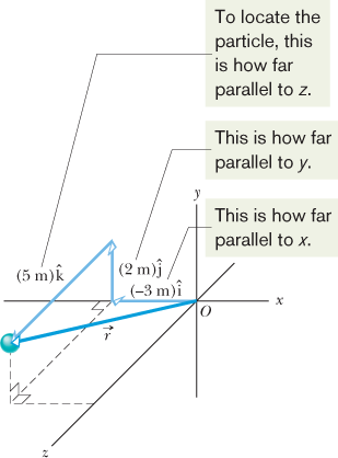
One general way of locating a particle (or particle-like object) is with a position vector

, which is a vector that extends from a reference point (usually the origin) to the particle. In the unit-vector notation of Module 3-2,

can be written

(4-1)

where

, and

are the vector components of

and the coefficients x, y, and z are its scalar components.

The coefficients x, y, and z give the particle's location along the coordinate axes and relative to the origin; that is, the particle has the rectangular coordinates

. For instance, Fig. 4-1 shows a particle with position vector

and rectangular coordinates

. Along the x axis the particle is

from the origin, in the

direction. Along the y axis it is

from the origin, in the

direction. Along the z axis it is

from the origin, in the

direction.

Figure 4-1
The position vector for a particle is the vector sum of its vector components.

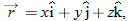
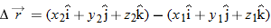
As a particle moves, its position vector changes in such a way that the vector always extends to the particle from the reference point (the origin). If the position vector changes—say, from

during a certain time interval—then the particle's displacement

during that time interval is

(4-2)

Using the unit-vector notation of Eq. 4-1, we can rewrite this displacement as

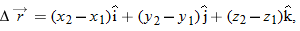
or as

(4-3)

where coordinates

correspond to position vector

and coordinates

correspond to position vector

. We can also rewrite the displacement by substituting

for

, and

for

(4-4)

Two-dimensional position vector, rabbit run

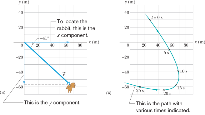
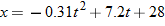
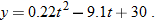
A rabbit runs across a parking lot on which a set of coordinate axes has, strangely enough, been drawn. The coordinates (meters) of the rabbit's position as functions of time t (seconds) are given by

(4-5)

and

(4-6)

(a)

, what is the rabbit's position vector

in unit-vector notation and in magnitude-angle notation?

KEY IDEA

The x and y coordinates of the rabbit's position, as given by Eqs. 4-5 and 4-6, are the scalar components of the rabbit's position vector

. Let's evaluate those coordinates at the given time, and then we can use Eq. 3-6 to evaluate the magnitude and orientation of the position vector.

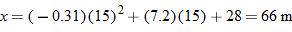
Calculations:

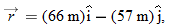
We can write

(4-7)

(We write

rather than

because the components are functions of t, and thus

is also.)

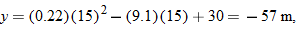
, the scalar components are

and

(Answer)

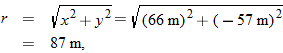
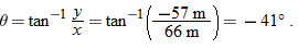
which is drawn in Fig. 4-2a. To get the magnitude and angle of

, notice that the components form the legs of a right triangle and r is the hypotenuse. So, we use Eq. 3-6:

(Answer)

and

(Answer)

Figure 4-2
(a) A rabbit's position vector at time . The scalar components of are shown along the axes. (b) The rabbit's path and its position at six values of t.

Check:

Although

has the same tangent as

, the components of position vector

indicate that the desired angle is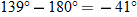

(b)	Graph the rabbit's path for t = 0 to . Graphing: We have located the rabbit at one instant, but to see its path we need a graph. So we repeat part (a) for several values of t and then plot the results. Figure 4-2b shows the plots for six values of t and the path connecting them.