| 4-2 | Average Velocity and Instantaneous Velocity |
|
Learning Objectives
After reading this module, you should be able to …
|
||||||||||||||||||
|
Key Ideas
|
||||||||||||||||||||

 ,
,  , and
, and  .
.
Average Velocity and Instantaneous Velocity
If a particle moves from one point to another, we might need to know how fast it moves. Just as in Chapter 2, we can define two quantities that deal with “how fast”: average velocity and instantaneous velocity. However, here we must consider these quantities as vectors and use vector notation.
If a particle moves through a displacement  in a time interval
  , then its average velocity
  is
is
or
This tells us that the direction of (the vector on the left side of Eq. 4-8) must be the same as that of the displacement (the vector on the right side). Using Eq. 4-4, we can write Eq. 4-8 in vector components as
For example, if a particle moves through displacement  in 2.0 s, then its average velocity during that move is
That is, the average velocity (a vector quantity) has a component of  along the x axis and a component of
  along the z axis.
in a time interval , then its average velocity is
|

|
|
(the vector on the left side of Eq. 4-8) must be the same as that of the displacement (the vector on the right side). Using Eq. 4-4, we can write Eq. 4-8 in vector components as
|
|
 in 2.0 s, then its average velocity during that move is
|
 along the x axis and a component of along the z axis.
When we speak of the velocity of a particle, we usually mean the particle's instantaneous velocity  at some instant. This is the value that approaches in the limit as we shrink the time interval to 0 about that instant. Using the language of calculus, we may write as the derivative
at some instant. This is the value that approaches in the limit as we shrink the time interval to 0 about that instant. Using the language of calculus, we may write as the derivative
|
|

Figure 4-3 shows the path of a particle that is restricted to the  plane. As the particle travels to the right along the curve, its position vector sweeps to the right. During time interval
, the position vector changes from
plane. As the particle travels to the right along the curve, its position vector sweeps to the right. During time interval
, the position vector changes from  to
to  and the particle's displacement is .
plane. As the particle travels to the right along the curve, its position vector sweeps to the right. During time interval
, the position vector changes from to and the particle's displacement is .
|
||||
|
||||
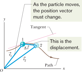
To find the instantaneous velocity of the particle at, say, instant t1 (when the particle is at position 1), we shrink interval to 0 about t1. Three things happen as we do so. (1) Position vector in Fig. 4-3 moves toward so that shrinks toward zero.  The direction of
  (and thus of ) approaches the direction of the line tangent to the particle's path at position 1. (3) The average velocity approaches the instantaneous velocity at t1.
to 0 about t1. Three things happen as we do so. (1) Position vector in Fig. 4-3 moves toward so that shrinks toward zero. The direction of (and thus of ) approaches the direction of the line tangent to the particle's path at position 1. (3) The average velocity approaches the instantaneous velocity at t1.
In the limit as  , we have
  and, most important here, takes on the direction of the tangent line. Thus, has that direction as well:
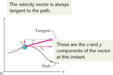
The result is the same in three dimensions: is always tangent to the particle's path.
, we have and, most important here, takes on the direction of the tangent line. Thus, has that direction as well:

The direction of the instantaneous velocity
of a particle is always tangent to the particle's path at the particle's position.
|
is always tangent to the particle's path.
To write Eq. 4-10 in unit-vector form, we substitute for  from Eq. 4-1:
This equation can be simplified somewhat by writing it as
where the scalar components of are
For example,  is the scalar component of along the x axis. Thus, we can find the scalar components of by differentiating the scalar components of .
from Eq. 4-1:
|
|
|
 are
are
|
|
 is the scalar component of along the x axis. Thus, we can find the scalar components of by differentiating the scalar components of .
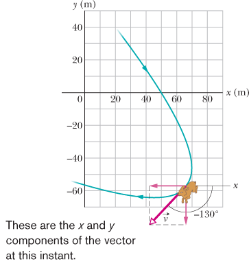
Figure 4-4 shows a velocity vector and its scalar x and y components. Note that is tangent to the particle's path at the particle's position. Caution: When a position vector is drawn, as in Figs. 4-1 through 4-3, it is an arrow that extends from one point (a “here”) to another point (a “there”). However, when a velocity vector is drawn,
as in Fig. 4-4, it does not extend from one point to another. Rather, it shows the instantaneous direction of travel of a particle at the tail, and its
length (representing the velocity magnitude) can be drawn to any scale.
and its scalar x and y components. Note that is tangent to the particle's path at the particle's position. Caution: When a position vector is drawn, as in Figs. 4-1 through 4-3, it is an arrow that extends from one point (a “here”) to another point (a “there”). However, when a velocity vector is drawn,
as in Fig. 4-4, it does not extend from one point to another. Rather, it shows the instantaneous direction of travel of a particle at the tail, and its
length (representing the velocity magnitude) can be drawn to any scale.
|
||||
|
||||
 Checkpoint 1 Checkpoint 1
|
 , through which quadrant is the particle moving at that instant if it is traveling (a) clockwise and (b) counterclockwise
around the circle? For both cases, draw
, through which quadrant is the particle moving at that instant if it is traveling (a) clockwise and (b) counterclockwise
around the circle? For both cases, draw 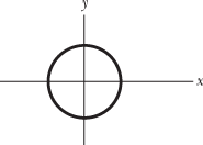

|
Sample Problem 4.02
Two-dimensional velocity, rabbit run
|
||||||||||||||||||||||||||||
 Two-dimensional velocity, rabbit run
 .
.
 . Similarly, applying the
 . Equation
 or
or  ?
?