Lab 1 - Force Table

Introduction

All measurable quantities can be classified as either a scalar or a vector. A scalar has only magnitude while a vector has both magnitude and direction. Examples of scalar quantities are the number of students in a class, the mass of an object, or the speed of an object, to name a few. Velocity, force, and acceleration are examples of vector quantities. The statement "a car is traveling at 60 mph" tells us how fast the car is traveling but not the direction in which it is traveling. In this case, we know the speed of the car to be 60 mph. On the other hand, the statement "a car traveling at 60 mph due east" gives us not only the speed of the car but also the direction. In this case the velocity of the car is 60 mph due east and this is a vector quantity. Unlike scalar quantities that are added arithmetically, addition of vector quantities involves both magnitude and direction. In this lab we will use a force table to determine the resultant of two or more force vectors and learn to add vectors using graphical as well as analytical methods.

Discussion of Principles

Vector Representation

As mentioned above, a vector quantity has both magnitude and direction. A vector is usually represented by an arrow, where the direction of the arrow represents the direction of the vector, and the length of the arrow represents the magnitude of the vector. In three-dimensions, a vector directed out of the page (or along the positive z-axis) is represented by (a circle with a dot inside it) and a vector directed into the page (or along the negative z-axis) is represented by (a circle with an × inside it). In mathematical equations a vector is represented as

A

. In some textbooks a vector is represented by a bold face letter A. The negative of a vector

A

is a vector of the same length but with a direction opposite to that of

A

. See Fig. 1 below.

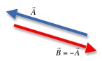
Figure 1: Vectors as arrows

The Cartesian coordinate system is used for graphical representation of vectors. The tail of the vector is placed on the origin and the direction of the vector is defined by an angle, θ (theta), between the positive x-axis and the vector, as shown in Fig. 2.

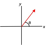
Figure 2: Graphical representation of a vector

Components of Vectors

An important technique when working with vectors mathematically is to break them down into their x and y components. In this example, we will consider the position vector

A

directed at an angle of 30° from the +x-axis and having a magnitude of 8.0 miles. From the head of the vector draw a line perpendicular to the x-axis and a second line perpendicular to the y-axis. We refer to these lines as the projections of the vector on to the x- and y-axes. The projection of the vector on to the y-axis gives the magnitude of the x-component of the vector (green line in Fig. 3 below) and the projection of the vector on the x-axis gives the magnitude of the y-component (red line in Fig. 3).

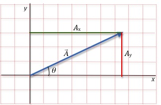
Figure 3: Breaking a vector into x and y components

Note that the green and red lines in the diagram above form two sides of a rectangle with the vector as the diagonal of the rectangle. We can also look at the above situation in two other ways as shown in Fig. 4.

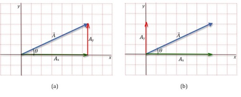
Figure 4: Representing components of a vector

In Fig. 4a we have a right triangle in which the vector is the hypotenuse, the side parallel to the x-axis (green arrow) is the x-component of the vector, and the side parallel to the y-axis (red arrow) is the y-component of the vector. Figure 4b is mathematically equivalent to Fig. 4a, but now

A_y

is drawn along the y-axis.

Finding components given the magnitude and direction of the vector

We know the direction of the

A_x

and

A_y

vectors, but to find their magnitudes we need to use some trigonometric identities. In Fig. 5 the hypotenuse represents the magnitude of the vector

A

and the other two sides of the right triangle represent the x and y components of the vector

A

.

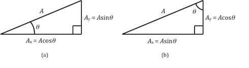
Figure 5: Finding the components of a vector

For any right triangle, we have the following trigonometric identities.

( 1 )

cos θ =

adjacent side

hypotenuse

( 2 )

sin θ =

opposite side

hypotenuse

Here, adjacent side refers to the side that is adjacent to the angle θ and opposite side refers to the side opposite to the angle θ. Let us consider the set-up in Fig. 5a. Using the definitions in Eqs. (1)

cos θ =

adjacent side

hypotenuse

and (2)

sin θ =

opposite side

hypotenuse

, we have

( 3 )

cos θ =

Ax

A

or A_x = A cos θ

( 4 )

sin θ =

Ay

A

or A_y = A sin θ

In Fig. 5b however, the angle θ is defined differently. In this case

( 5 )

sin θ =

Ax

A

or A_x = A sin θ

( 6 )

cos θ =

Ay

A

or A_y = A cos θ

It is a common mistake to assume that

A_x

is always the cosine component and

A_y

is always the sine component. However, this will depend on which of the two angles in the right triangle is defined as θ. Note that

A_x

is adjacent to the angle θ in Fig. 5a, while in Fig. 5b

A_y

is adjacent to the angle θ. In Fig. 3, the magnitude of

A

is 8.0 miles and its direction is 30° above the +x-axis. So you find the magnitude of

A_x

and

A_y

as follows:

( 7 )

A_x = A cos θ = 8.0 miles * cos(30°) = 6.9 miles

( 8 )

A_y = A sin θ = 8.0 miles * sin(30°) = 4 miles

In other words, if you were walking, you could walk 6.9 miles due east (along the +x-axis) then 4 miles due north (along the +y-axis). This would bring you to the same destination if you were to walk 8 miles in the direction that is 30° from the +x-axis.

Finding the magnitude and direction of the vector from the components

If you do not know the magnitude or direction of the vector, but know the distances traveled in the x and y directions, you can use the Pythagorean theorem to find the hypotenuse, which is the total distance traveled.

( 9 )

A² = A_x² + A_y² or A =

Ax2 + Ay2

The direction of the vector can be found using one of the following equations.

( 10 )

θ = sin⁻¹

Ay

A

( 11 )

θ = cos⁻¹

Ax

A

( 12 )

θ = tan⁻¹

Ay

Ax

Some Basic Properties of Vectors

Two vectors are equal if they have the same magnitude and direction. So, on paper, you can slide a vector to a different location, but as long as you keep the same length and orientation for the arrow, the two vectors will be equal. In Fig. 6a the two vectors

A

and

B

have the same length and orientation. The negative of a vector has the same length but with the direction reversed, as shown in Fig. 6b. A vector multiplied by a scalar will be a vector in the same direction as the original vector but with a different magnitude. In Fig. 6c p is a scalar. The vector

B

has the same direction as

A

but it is longer by a factor of p with p greater than 1. If p was less than 1, then

B

would be shorter than

A

.

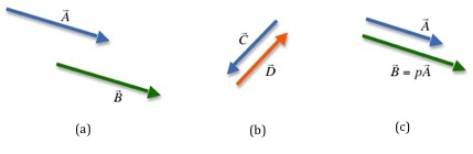
Figure 6: Vector properties

Graphical Method of Adding Vectors

Consider two vectors

A

and

B

oriented as shown in Fig 7. We would like to find the sum and difference of the two vectors. Unlike adding scalar quantities, in this case we need to consider both magnitude and direction.

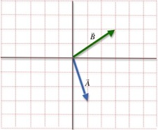
Figure 7: Two vectors

To add two vectors, slide the second vector so that its tail is at the head of the first vector. The sum of the two vectors is a vector drawn from the tail of the first vector to the head of the second vector. In Fig. 8a,

B

is moved so that its tail is at the head of

A

. Note that the direction of

B

does not change. The red arrow gives the sum

R = A + B

. Addition is commutative, so you will get the same result by moving

A

to the head of

B

. To find the difference of two vectors, we can take the negative of the second vector and add it to the first vector following the steps described above for addition. In other words,

A − B = A + (−B)

. This is illustrated in Fig. 8b.

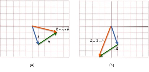
Figure 8: Sum and difference of two vectors

Analytical Method of Adding Vectors

Addition or subtraction of vectors involves breaking up the vectors into its components and then performing the addition or subtraction to the x and y components separately.

( 13 )

R_x = A_x + B_x

( 14 )

R_y = A_y + B_y

Now using Eqs. (9)

A² = A_x² + A_y² or A =

Ax2 + Ay2

and (12)

θ = tan⁻¹

Ay

Ax

we can find the magnitude and direction of the resultant vector

R

. This process will be the same if you are adding more than two vectors or subtracting vectors. In Fig. 5a,

A_x = 1

and

B_x = 3

giving

A_x

+

B_x = 4;

A_y = −3

and

B_y = 2

giving

A_y + B_y = −1.

These values agree with the x and y components of the red arrow in Fig. 5a. In the case of subtraction

A_x − B_x = −2; A_y − B_y = −5

. These values agree with the x and y components of the red arrow in Fig. 5b.

Force vectors

In this lab you will deal with force vectors. In addition to the general properties of vectors discussed thus far in this lab, the following definitions will be useful as you work through this lab. The vector sum of two or more forces is the resultant. The resultant can, in effect, replace the individual vectors. The equilibrant of a set of forces is the force needed to keep the system in equilibrium. It is equal and opposite to the resultant of the set of forces.

Objective

The objective of this experiment is to find the equilibrant of one or more known forces using a force table and compare the results to that obtained by analytical method.

Equipment

Procedure

Given two force vectors you will determine the third force that will produce equilibrium in the system. This third force is known as the equilibrant and it will be equal and opposite to the resultant of the two known forces. You will use a force table as shown in Fig. 9, and work with force vectors. The force table is a circular platform mounted on a tripod stand. The three legs of the tripod have adjustable screws that can be used to level the circular platform. The circular platform has angle markings, in degrees, on its surface. Two or more pulleys can be clamped at any location along the edge of the platform. In this lab we will use three pulleys. Three strings are attached to a central ring and then each string is passed over a pulley. Masses are added to the other end of the strings.

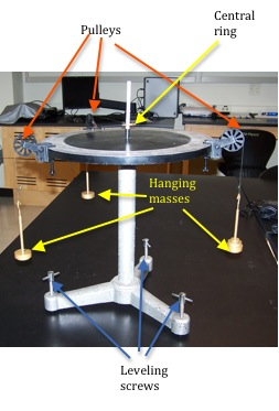
Figure 9: Force table

The hanging masses will produce a tension force in each string. The masses are directly proportional to the gravitational force (which you will learn about later in the course). The tension force in each string is equal to the gravitational force. For example, doubling the mass doubles the force, etc. When the forces are balanced, the ring will be positioned at the exact center of the table. When the forces are not balanced, the ring will rest against one side of the central post. Note: The force due to each hanging mass will be mg where g is the acceleration due to gravity. To make it easier to read the angles, assume the x-axis to be from the 180° mark to the 0° mark, with 0° being the positive x direction, and the y-axis to be from the 270° mark to the 90° mark with 90° being the positive y direction. See Fig. 10.

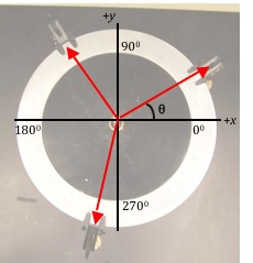
Figure 10: Force table with axes

Procedure A: Finding the Equilibrant of Two Known Forces

Procedure B: Determining the Placement of Two Unknown Forces

Copyright © 2010 Advanced Instructional Systems, Inc. and North Carolina State University. | Credits