Lab 2 - Uniformly Accelerated Motion

Introduction

All objects on the earth's surface are being accelerated toward the center of the earth at a rate of 9.81m/s². This means that if you raise an object above the surface of the earth and then drop it, the object will start from rest and its velocity will increase by 9.81 meters per second for each second it is falling toward the earth's surface until it strikes the surface.

Discussion of Principles

In this experiment you will measure, with the aid of computer-based instruments, the position of a falling body as a function of the time elapsed since it was released. We adopt the downward direction as positive, and we denote displacements in that direction by

. When air resistance is neglected, the body is said to be in free fall, and its acceleration

is constant. Consider an object at position

y₁

at some initial time

t₁

. At a later time

t₂

the object is at location

y₂

. The average velocity

v₁₂

for this object as it travels between these two points will be

( 1 )

v₁₂ =

(y₂ − y₁)

(t₂ − t₁)

Similarly, the average velocity

v₂₃

during the next time interval (that is, between the instants

t₂

and

t₃

) is

( 2 )

v₂₃ =

(y₃ − y₂)

(t₃ − t₂)

If the acceleration is uniform or constant, the velocity at exactly the mid point of the time interval is the average velocity. This means that if the acceleration is constant, the instantaneous velocity is exactly equal to the average velocity at the midpoint of the time interval that is being examined. Even if the acceleration were not uniform, this would be a close approximation if the interval of time were short. So

v₂₃

would occur at the midpoint of the time interval given by

( 3 )

t₂₃ =

(t₃ + t₂)

With these two average velocities and times we can calculate an average acceleration

( 4 )

a =

Δv

Δt

(v₂₃ − v₁₂)

(t₂₃ − t₁₂)

where

Δv

and

Δt

denote the change in velocity and time, respectively. For an object moving with constant velocity, a plot of distance versus time would be a straight line with a constant slope like the graph in Fig. 1a below. Since distance is plotted on the vertical axis and time is plotted on the horizontal axis, the slope is

Δ(Distance)/Δ(Time)

or the average velocity. Here the average velocity is the same as the instantaneous velocity at any given time.

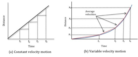
Figure 1: Plot of distance versus time

Figure 1b shows a plot of position versus time for an object moving with increasing velocity. Here we can draw a graph where we connect the points with the solid lines indicated by the red lines in Fig 1b. If we were to measure the position of the object over smaller time intervals we would see a smoother curve as indicated by the blue curve. The average velocity between two points

x₁

t₁

and

x₂

t₂

, is given by the slope of the straight line connecting these two points. Now consider the velocity versus time version of this graph shown in Fig.2. The average velocities intersect with the instantaneous velocities at the midpoint of the two time measurements. The average of two points is the midpoint of the two points. So when we take the average of

t₂

and

t₃

we find the time at the half-way point. Here we refer to this time as

t₂₃

. As shown in Fig.2, the instantaneous velocity and the calculated average velocity have the same value at this average time,

t₂₃

. This is why we use the average time and average velocity when calculating the acceleration.

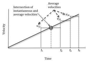
Figure 2: Graph showing instantaneous and average velocities

The kinematic equations are derived from the definitions of average velocity and acceleration discussed above for a uniformly accelerating object. These equations provide a useful way to evaluate the motion of an object moving with constant acceleration. For one-dimensional motion, the kinematic equations are

( 5 )

v_f = v_i + aΔt

( 6 )

x_f = x_i + v_iΔt +

a(Δt)²

( 7 )

v_f² = v_i² + 2aΔx

where

v_i

and

v_f

are the initial and final velocities when the object is at positions,

x_i

and

x_f

respectively,

Δt

is the elapsed time and

the constant acceleration for this motion. In summary, you can find the acceleration by considering data from two consecutive time intervals:

1
Calculate the average velocity
v₁₂
for the first time interval from the distance
y₂ − y₁
traveled during the time interval
t₂ − t₁
. This is the instantaneous velocity at
t₁₂
.
2
Calculate the average velocity
v₂₃
for the second time interval from the distance
y₃ − y₂
traveled during the time interval
t₃ − t₂
. This is the instantaneous velocity at
t₂₃
.
3
Calculate the acceleration
a
from the two velocities
v₁₂
and
v₂₃
and the elapsed time
t₂₃ − t₁₂
for these velocities.

Objective

The objective of this experiment is to measure the position of an object in free fall as a function of time and to determine the acceleration due to gravity.

Equipment

Picket fence
Photogate
Signal Interface
DataStudio software
Computer
Meter stick

Procedure

A picket fence, which is a piece of clear acrylic (also known as Plexiglas or Lucite) covered with equally spaced black bands, will be dropped through a photogate connected to a computer. See Fig. 3. A beam of light passes from one prong of the photogate to the other. The signal interface monitors the beam and reports, to the computer, the time at which the beam was broken.

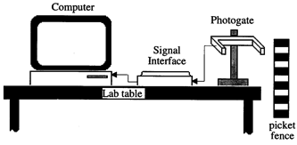
Figure 3: Experimental set-up

From these instants of time the intervals of time between bands can be found. These time intervals, along with the distances between the bands, will allow you to calculate the average velocities of the fence during the time intervals. You can calculate the average velocity

v_n,n+1

of the fence during a given time interval after measuring, the distance

y_n+1 − y_n

from the first edge of one black band to the first edge of the next black band and the time interval

t_n+1 − t_n

it took for the fence to fall that distance.

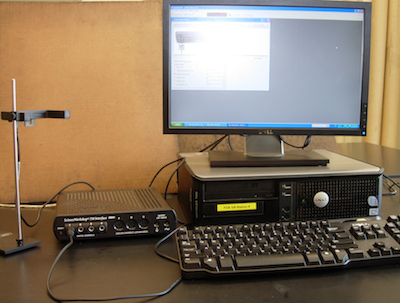
Figure 4: Photo of experimental setup

Procedure A: Set-up and data acquisition

The black bands on the picket fence should be equally spaced and of equal width. Use a meter stick to measure the distance from the leading edge of the first black band to the leading edge of the second black band, as shown in Fig. 5.

Repeat this measurement at other locations on the picket fence and take the average value of the band width

, where

c = y_n+1 − y_n

, for all values of

. Enter this value on the worksheet.

Figure 5: Picket fence

Open the appropriate Pasco Capstone file for this lab. A screen similar to Fig. 6 is displayed. Note that Table 1 will be next to the Experiment Setup window.

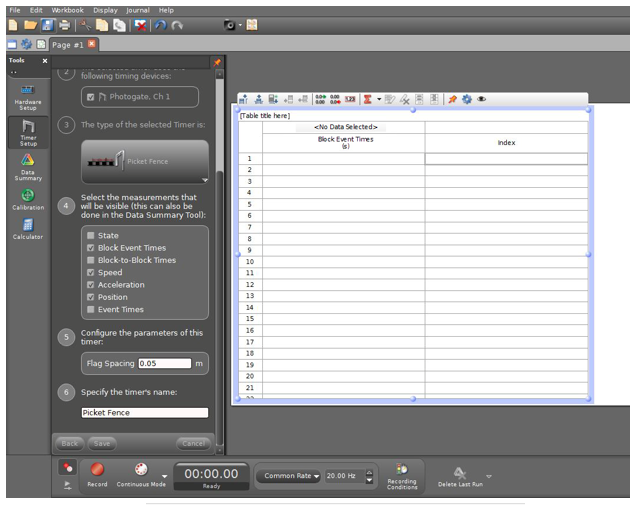
Figure 6: Opening screen for free fall experiment

You must enter the value of the picket spacing in the block labeled Flag Spacing. Enter the value in meters, and then click the Save button below.

Position the photogate near the edge of a table so the picket fence can fall through the photogate beam. Place a piece of clothing or similar cushioning material beneath the photogate so that the picket fence is not damaged when it hits the floor.

When you are ready to record data, click the Record button. See Fig. 7. Data recording will automatically begin when the photogate beam is first interrupted by the falling picket fence.

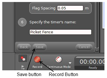
Figure 7: Recording data

Position the fence just above the photogate, and release it. After the fence passes through the photogate, click the Stop button. The table, which was empty in Fig. 6, will now be filled with data that contains two columns. The first column contains the instants of time (measured in seconds) that the leading edges of the dark bands passed through the photogate and the second column gives the counts, i.e., the number of times the beam was interrupted. See Fig. 8.

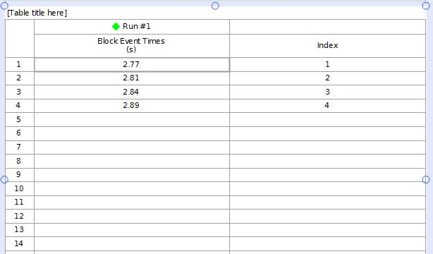
Figure 8: Data table for falling picket fence

Using Excel, create a table similar to Data Table 1 on the worksheet. See Appendix F. Refer to Eqns 1, 2, 3, and 4 as you complete Data Table 1.

Checkpoint 1:
Ask your TA to check your Excel worksheet before proceeding.

After your TA has checked your work record the numbers from your Excel sheet into Data Table 1 on the worksheet.

Determine the average of the five acceleration values and enter it on the worksheet. See Appendix E.

Any object (of sufficient mass per unit volume to reduce air drag) near the earth's surface will accelerate toward the earth with the constant acceleration,

. The accepted value for this acceleration is 9.81 m/s². Since the only force acting on the picket fence during its free fall was gravity, the acceleration you found should be the acceleration of gravity.

Compute the percent error between your average acceleration and the accepted value of the acceleration due to gravity and enter it on the worksheet. See Appendix B.

Procedure B: Plot of velocity versus time

Using Excel, plot a graph of the velocity of the falling fence as a function of time. See Appendix G. Use the data from column 3 of your table for the velocities, and use column 2 for the time instants.

Add a linear trendline to your plot and determine the average acceleration from the slope. See Appendix H. Enter this value on the worksheet.

Calculate the percent error between the value of the acceleration obtained from the slope and the accepted value of the acceleration due to gravity

. Enter this value on the worksheet.

Checkpoint 2:
Ask your TA to check your graph and calculations.

Procedure C: Predicting velocity using kinematics

Now that you have an experimental value of acceleration you can use kinematics to make predictions about the velocity and position of the fence at any time during its descent. You will predict the average speed of the fence when it is dropped from a given height as described in step 16 below. You will then test your prediction by dropping the fence from that height and finding the average velocity from this new set of data.

The fence is held at a height of 0.15 m, measured from the top of the first black band to the laser beam and released from rest. Using kinematics and the value of acceleration from the slope of your graph in step 14, predict how fast the fence will be traveling when the first black band interrupts the laser beam.

Now confirm your prediction. Hold the fence so that it matches the conditions used for the prediction (i.e. the top of the first black band is 0.15 m above the photogate). Click the Start button, and then release the fence. Using the first two time values, find the average velocity of the fence, and enter it on the worksheet. It should be close to your predicted value.

Calculate the percent difference between the predicted and experimental values and record it on the worksheet.

Checkpoint 3:
Ask your TA to check your graph and calculations.