Lab 2 - Electric Field and Electric Potential

Introduction

Physicists use the concept of a field to explain the interaction of particles or bodies through space, i.e., the "action-at-a-distance" force between two bodies that are not in physical contact. The earth modifies the surrounding space such that any body with mass, such as the moon, is attracted. The gravitational field gets weaker as you go farther away from the source but never completely disappears. An electron modifies the space around it in such a way that other particles with like charge are repelled, while particles with the opposite charge are attracted. Like the gravitational field, the electric field gets weaker with distance from the source but is never completely gone. Any charge placed in an electric field will experience a force, as will any mass placed in a gravitational field. Just as mass in a gravitational field has some potential energy, so does a charge in an electric field. In this lab, we will examine some aspects of electric field and electric potential.

Discussion of Principles

A charged body experiences a force

whenever it is placed in an electric field

The vector relationship between the force and the electric field is given by

( 1 )

= qE

The magnitude of the force divided by the magnitude of the charge q on the body is numerically equal to the magnitude of the electric field.

( 2 )

= F

From Eq. (1), we see that the direction of the electric field vector at any given point is the same as the direction of the force that the field exerts on a positive test charge located at that point. A positive test charge will be repelled by a positive charge and attracted by a negative charge. Therefore electric field lines start on positive charges and end on negative charges. The number of lines starting from a positive charge or ending on a negative charge is proportional to the magnitude of the charge. The electric field at any point is tangential to the electric field lines. The magnitude E of the electric field strength is proportional to the number of electric field lines per unit area perpendicular to the lines. A positive charge placed in an electric field will tend to move in the direction of the electric field lines and a negative charge will tend to move opposite to the direction of the electric field lines.

Work, Potential Energy, and Electrostatic Potential

Work is done in moving a charged body through an electric field. The amount of work W done depends on the electric field, the magnitude of the charge and the displacement

that the charge makes through the field. When the displacement is so small that the electric field can be assumed uniform in the region through which the charge moves, the work W is given by the dot product of the force and displacement vectors.

( 3 )

W = F

· d

= q E

· d

The negative of the work done by the electric force is defined as the change in electric potential energy U of the body. Put another way, it is the difference in the potential energies

ΔU

associated with the starting and ending positions.

( 4 )

−W = ΔU = (U_final − U_initial)

The electrostatic potential V is defined as the electric potential energy of the body divided by its charge:

V = U/q.

In terms of electrostatic potential, the work done by the electric field is

( 5 )

W = −qΔV

where

ΔV = V_final − V_initial

is the potential difference. The magnitude of the electric field can also be determined from Eqs. (3) and (5).

( 6 )

E =

ΔV

d cos θ

where

is the angle between the field and displacement vectors. When a charged particle moves in an electric field, if its electric potential energy decreases, its kinetic energy will increase. In other words, the total energy is conserved. A positive charge placed in an electric field will tend to move in the direction of the field. The work done by the electric field in this case will be positive as the field and the displacement vectors are in the same direction and the dot product of the two vectors will be positive as shown in Fig. 1(a). Note that the velocity vector indicates the direction of the displacement vector for the charge.

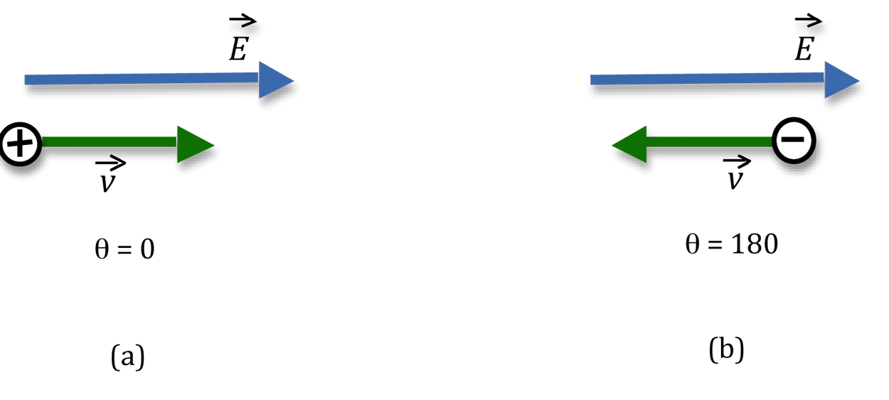
Figure 1: Motion of charges in an electric field

From Eq. (4), we see that the change in electric potential energy will be negative in this case. It will therefore lose electric potential energy and gain kinetic energy. This tells us that electric potential decreases in the direction of the electric field lines. A positive charge, if free to move in an electric field, will move from a high potential point to a low potential point. Now consider a negative charge placed in an electric field as shown in Fig. 1(b). It will tend to move in a direction opposite to the electric field and accelerate as it does so. The work done by the electric field will be

( 7 )

W = (−q)E

· d

= −qEd cos 180° = qEd.

Again, note that the work done by the electric field is positive and the negative charge will lose electric potential energy and gain kinetic energy as it moves against the field. A negative charge, if free to move in an electric field, will move from a low potential point to a high potential point. To move a positive charge against the electric field, work has to be done by you or a force external to the field. The charge is forced to move from a low potential point to a high potential point and the work done by the external force is negative. The reverse will be true for a negative charge. As in the case of the gravitational field, the zero point of the electric potential is chosen arbitrarily. In general, the zero point is at infinity. Very often, the zero point is the ground or a conductor that is directly connected to the ground.

Equipotential Lines and Electric Field Lines

Consider the field due to a single point charge. A point in this space near the source of the field (i.e., near the point charge), and another point far from the source of the field are at different potentials. This is true even if no charges reside at the two points. In Fig. 2, points A and B are at different potentials due to the electric field of the positive charge.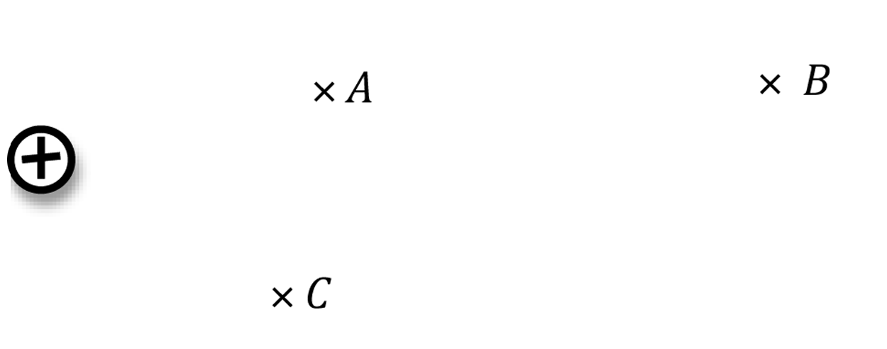

Figure 2: Electric potential at different points in a field

All fields have certain points that are at the same potential. For example, when a point charge is the source of the field, then any two points that are the same distance from the point charge (points A and C in Fig. 2) will be at the same potential. There are an infinite number of points—all lying on the same sphere—that are at the same distance, all of which are at the same potential. In three dimensions these points form a surface, called an equipotential surface. In two dimensions—say, the equatorial plane of the sphere—the circle (equator) where the sphere intersects the plane is an equipotential line; the potential difference between any two points on this line is zero. It follows from Eq. (4) that no work is done in moving a charge along an "equipotential" i.e., an equipotential line or surface. Eq. (4) also tells us that no work is done when the displacement and the field are perpendicular to one another. Therefore, the electric field vectors must be perpendicular to the equipotentials.

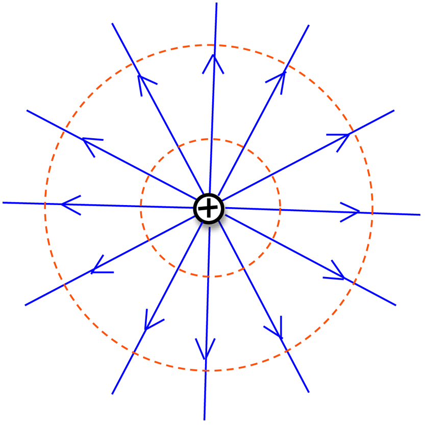
Figure 3: Electric field lines and equipotential lines

Fig. 3 shows a few of the electric field lines (blue lines with arrows) for a positive charge. The dashed red circles are two of the many equipotential circles. At any given point on one of these circles, the tangent to the circle will be perpendicular to the electric field line direction at that point. Because it is not simple to find the electric field lines directly, you will in this experiment first locate the equipotential lines, and then draw the field lines by knowing that they are perpendicular to the equipotential lines.

Objective

The objective of this experiment is to draw equipotential lines for four different charge configurations. You will then use these equipotential lines to map the electric field lines for each configuration.

Equipment

PASCO Scientific field mapper
Signal interface with power output
Electrodes
Voltage probe
DataStudio software

Procedure

Please print the worksheet for this lab. You will need this sheet to record your data.

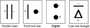
You will use the PASCO scientific field mapper, which consists of a sheet of carbon-impregnated paper. The electrodes or charged bodies are formed by a line of conductive ink, which has been drawn on the paper and then allowed to dry. You will be supplied with four electrode configurations already drawn out on conductive paper, which match the copies provided on the worksheet. The patterns are shown in Fig. 4 below.

Figure 4: Electrode patterns

Do not draw on the carbon-impregnated paper. You will use the field mapper to determine equipotential points and transfer these locations to the corresponding copy provided on the worksheet. The original conducting paper and the copy have the same number of fiducial marks, but they are closer together on the copy than on the original, i.e., the scale is different.

Insert the voltage probe (the plug with a red and a black lead) into the analog channel A of the PASCO ScienceWorkshop 750 interface and connect two wires to the output of the interface. This will serve as your voltmeter. Your interface should have connections similar to those shown in Fig. 5.

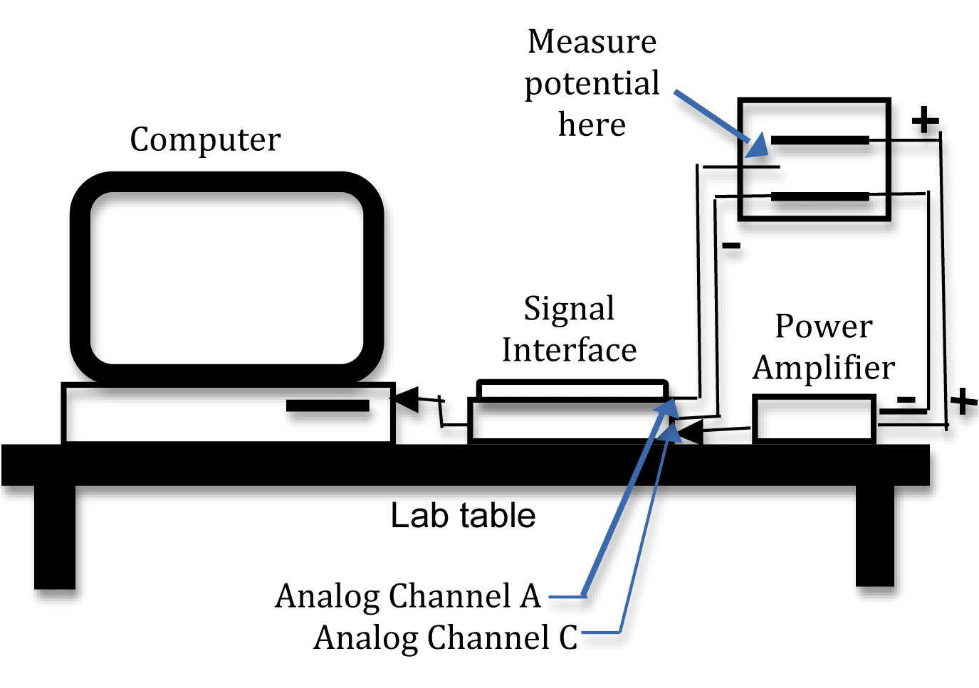
Figure 5: Schematic of connections to computer interface

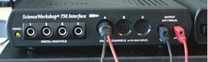
Figure 6: Photo of connections to computer interface

Procedure A: Parallel Lines

Connect the output wires from the signal interface to the bolts on the conduction paper. Then connect one of the wires from the voltage probe to one of the output wires. The second wire from the voltage probe will be placed at various locations around the configuration and will measure the potential difference between that location and the electrode connected to the first voltage probe wire. Your electrode connections should look like those shown in Fig. 7.

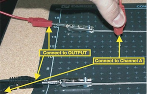
Figure 7: Electrode connections

Open the appropriate DataStudio file associated with this lab. Fig. 8 shows the opening screen in DataStudio. You will see the "Experiment Setup" window, the "Signal Generator" window and the "Digits" window.

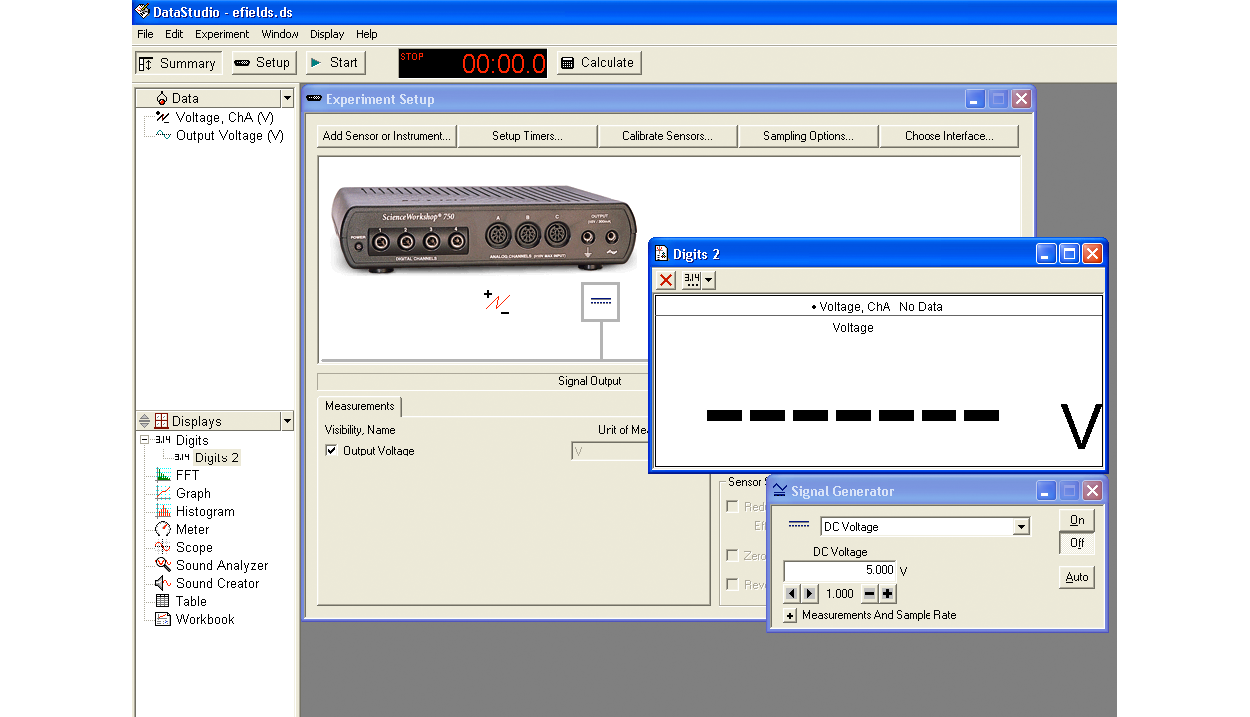
Figure 8: Opening screen view of DataStudio

You may need to reposition the "Experiment Setup" window in order to see the other windows.

The "Signal Generator" window is shown in Fig. 9. Make sure the DC button of the icon is not already highlighted. Set the DC voltage to 5 V using the + and – buttons (+ to increase the value and – to decrease the value) to the right of the voltage setting.

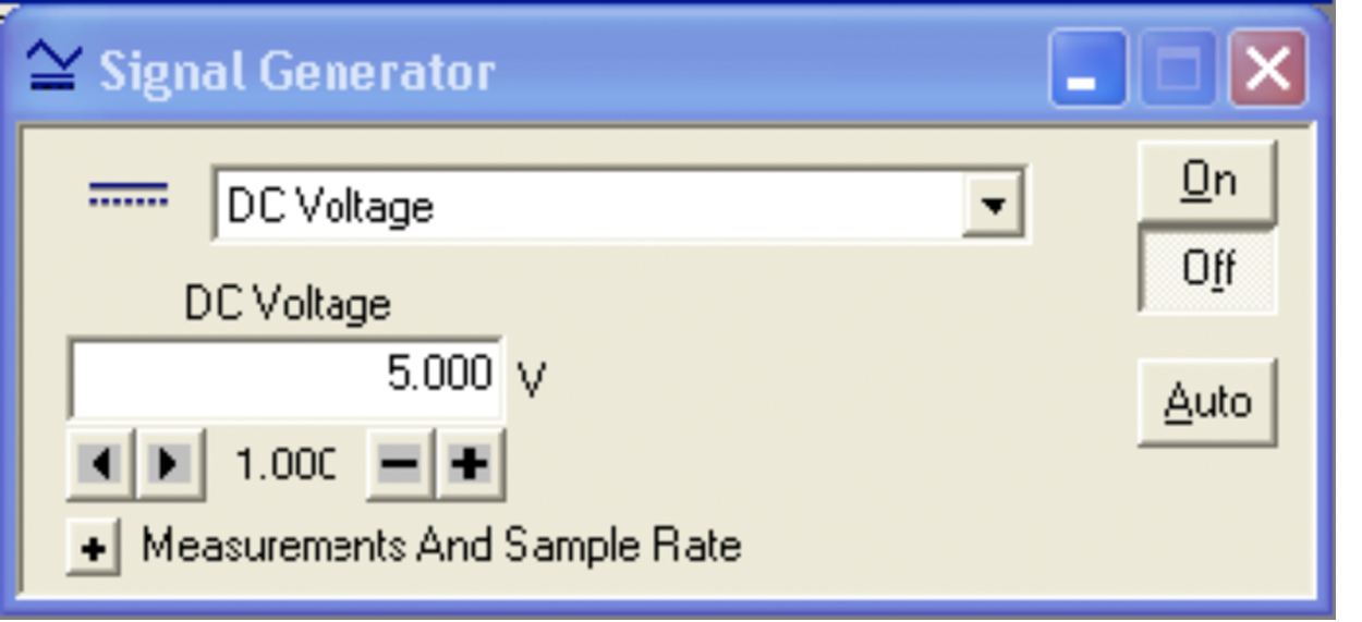
Figure 9: "Signal Generator" window

Turn on the signal generator by clicking ON.

To monitor the signal, click Start in the main window.

Use the free lead (red) from the signal interface to probe the potential at various points on the paper around the electrodes. Do not drag the voltage probe across the paper, as that damages the paper. Lift the probe after each measurement and then move it to another place on the paper to make the next measurement. The potential is displayed on the voltmeter in DataStudio.

Place the probe at different points in the space between the two parallel lines and determine the direction in which the voltage increases. From this, determine which of the two parallel lines is at a higher potential and mark this on the parallel lines configuration on your worksheet.

If necessary, reorient your mapping paper so the positive line is to the left.

Trace five equipotential lines until they close or leave the graph. Determine the position of the probe from the fiducial marks on the paper, and transfer the coordinates of this position to the corresponding copy.

Your graph should have five equipotential lines which pass through the space between the electrodes and out to the edges of the paper. Be sure to label the voltage of each of the equipotential lines.

Measure the potentials at the five locations A, B, C, D, and E. Record these voltage values in Data Table 1 on the worksheet.

Measure the distance of these five locations from the positive line, and record these in Data Table 1.

Construct five electric field lines connecting one electrode to the other. Draw arrows indicating the direction of the field lines.

Complete the calculations for Data Table 2 on the worksheet.

Checkpoint 1:
Ask your TA to check your field lines and calculations before proceeding.

Procedure B: Point and Line

Place the probe at different points in the space between the electrodes to determine the direction in which the voltage increases. From this determine the high potential end of the configuration and mark this on the copy in your worksheet.

If necessary, reorient your mapping paper to match that shown for this configuration in Fig. 4.

Repeat steps 11 and 12 for the point and line configuration. Determine equipotential points on either side of the line as well as all the way around the point.

Construct five electric field lines connecting one electrode to the other and draw arrows indicating the direction of these field lines.

Note: To draw a line perpendicular to a curve, consider the tangent to the curve at the point.

Measure the potentials at two points along the electric field line close to and on either side of the location A. Record these voltage values in Data Table 3 on the worksheet.

Measure the distance between these two points and record this on the worksheet.

From the values obtained in steps 21 and 22 calculate the electric field strength at location A using Eq. (6).

Repeat steps 21 through 23 for the other four locations B, C, D, and E.

Complete the calculations for Data Table 3 on the worksheet.

Checkpoint 2:
Ask your TA to check your field lines and measurements before proceeding.

Procedure C: Dipole

Repeat steps 17 through 25 for the dipole configuration. Determine equipotential points in the space between the two points as well around the points.

Complete the calculations for Data Table 4 on the worksheet.

Checkpoint 3:
Ask your TA to check your field lines and measurements before proceeding.

Procedure D: Line and Triangle

Repeat steps 17 through 25 for the line and triangle configuration. Determine equipotential points in the space inside the triangle as well as outside it.

Complete the calculations for Data Table 5 on the worksheet.

Checkpoint 4:
Ask your TA to check your field lines and measurements.