Lab 9 - AC Circuits

Introduction

The study of alternating current (AC) in physics is very important as it has practical applications in our daily lives. As the name implies, the current and voltage change directions periodically at a fixed frequency. In the United States, this frequency is usually 60 Hz, while European countries use 50 Hz. The alternating current is transmitted at high voltage and low amperage on the main transmission lines so that power loss may be kept to a minimum. The voltage is stepped down several times before it enters your home. Most electric appliances need a voltage of 120 V, though some appliances like heating and air conditioning equipment, water heaters, and ovens require 240 V. Earlier in this course you may have studied the behavior of resistors, capacitors, and inductors in a circuit with a dc source or, as in the case of discharging a capacitor, with no source at all. In this lab you will analyze the relationship between current and voltage when these elements are connected in a circuit with an ac source of emf.

Discussion of Principles

The voltage of an AC source varies sinusoidally with time with a frequency f given by

( 1 )

ω = 2πf

where

is the angular frequency measured in radians/second. The current delivered by an AC source is also sinusoidal.

( 2 )

I = I₀cos(2πft)

where I₀ is the maximum or peak current and t is the time.

Resistance in an AC Circuit

Consider the resistor R connected to an AC source of emf as shown in Fig. 1(a).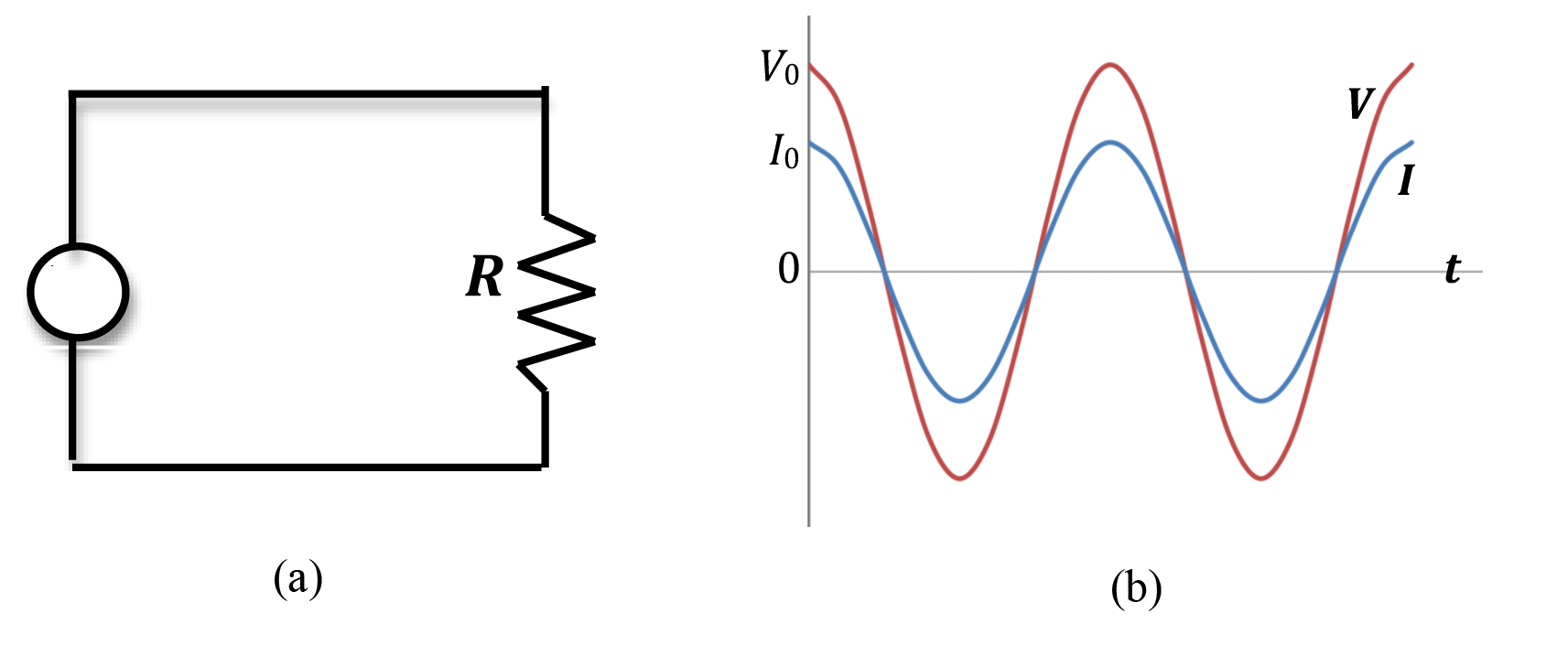

Figure 1: Current and voltage in a resistor connected to an AC source of emf

The current through the resistor is given by Eq. (2) and the voltage across the resistor obeys Ohm's Law.

( 3 )

V = IR = I₀cos(2πft)R = V₀cos(2πft)

where the peak voltage across the resistor is

V₀ = I₀R.

Fig. 1(b) shows the plots of current and voltage as a function of time t. Note that both the current and voltage reach peak values at the same instant of time and they are both zero at the same instant of time. Therefore, we say that the current and voltage are in phase or the phase difference is zero.

Inductance in an AC Circuit

Consider the inductor L connected to an AC source of emf as shown in Fig. 2(a).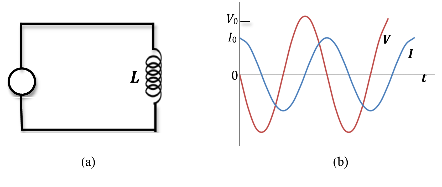

Figure 2: Current and voltage in an inductor connected to an AC source of emf

The current in the circuit is given by Eq. (2) and the voltage across the inductor is given by

( 4 )

V_L = L

This is the emf induced in the coil due to the changing current. Combining Eq. (2) and Eq. (4) gives

( 5 )

V_L = −V₀sin(2πft)

where

V₀

is the peak voltage. Fig. 2(b) shows the plots of current and voltage as a function of time t. In this case, when the voltage is positive maximum, the current is zero and in the process of increasing. When the voltage is negative maximum, the current is decreasing. The current reaches its maximum value 1/4 cycle after the voltage reaches its maximum. Therefore, we say that the voltage leads the current by 90° or the current lags behind the voltage by 90°. Eq. (5) can be written as

( 6 )

V_L = V₀cos(2πft + φ)

where the phase difference

φ = π/2.

The current and voltage are related by an equation similar to Ohm's Law with

( 7 )

V_L = IX_L

where

X_L

is known as the inductive reactance, is measured in units of ohms, and is given by

( 8 )

X_L = 2πfL= ωL.

Capacitance in an AC Circuit

Consider the capacitor C connected to an AC source of emf as shown in Fig. 3(a).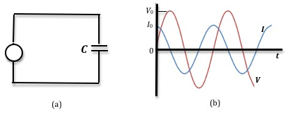

Figure 3: Current and voltage in a capacitor connected to an AC source of emf

The current in the circuit is given by Eq. (2) and the voltage across the capacitor is given by

( 9 )

V_C =

where the charge Q on the capacitor plates is related to the current by

( 10 )

I =

Combining Eqs. (2), (9), and (10), we get

( 11 )

V_C = V₀sin(2πft)

where

V₀

is the peak voltage. Fig. 3(b) shows the plots of current and voltage as a function of time t. In this case, the current reaches its maximum value 1/4 cycle before the voltage reaches its maximum. Therefore, we say that the voltage lags behind the current by 90° or the current leads the voltage by 90°. The voltage can be written as

( 12 )

V_L = V₀cos(2πft − φ)

where the phase difference

φ = π/2.

The current and voltage are related by an equation similar to Ohm's Law with

( 13 )

V_C = IX_C

where X_C is known as the capacitive reactance given by

( 14 )

X_C =

2πfC

ωC

Here X_C is measured in units of ohms.

RLC Circuit

A basic RLC circuit is shown in Fig. 4 with a capacitance C, an inductor L, and a resistor R connected in series.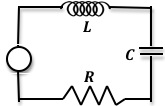

Figure 4: A simple RLC circuit

The voltage from the AC source is given by

( 15 )

V = V_R + V_C + V_L.

Note that the peak voltage

V₀

of the source will not equal the sum of the individual peak voltages of the three elements. This is due to the fact that the voltages across the resistor, capacitor, and inductor do not reach their peak values at the same time. The total impedance Z of the RLC circuit is given by

( 16 )

Z =

(X_C − X_L)² + R²

Ohm's Law for this circuit as well as for each component is then the following.

( 17 )

V₀ = I₀Z

( 18 )

V_R = IR

( 19 )

V_C = IX_C

( 20 )

V_L = IX_L

The applied voltage and the current are generally out of phase, and the phase difference is given by

( 21 )

φ = tan⁻¹

X_C − X_L

Since the impedance depends on frequency, the current varies with frequency as well, even when the voltage amplitude is constant. According to Eq. (17), the current will be at a maximum when the impedance is at a minimum. This occurs when

X_L − X_C = 0,

i.e., when

( 22 )

ω =

This frequency at which the current is maximum is known as the resonant frequency of the circuit. Fig. 5 is a graph of the current versus the frequency for a particular value of R.

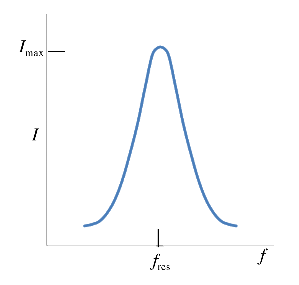
Figure 5: Plot of current versus frequency

At resonant frequency, the impedance is purely resistive. For very small values of R the circuit is referred to as an LC circuit and the energy oscillates between the inductor and the capacitor. Of course, a little bit of energy will be dissipated through the resistor. Applications of the phenomenon of resonant frequency include radio and TV sets where a varying L or C value is used for tuning to a particular station.

Objective

The purpose of this experiment is to study resonance in a series RLC circuit by measuring and plotting amplitude of the voltage versus frequency as well as to observe the variation in phase angle for values of the frequency on either side of the resonant value.

Equipment

PASCO circuit board
Capstone software
Signal interface with power output
Connecting wires
Multimeter

Procedure

Please print the worksheet for this lab. You will need this sheet to record your data.

Procedure A: Determining Resonant Frequency

Turn off the power amplifier and the signal interface.

Construct the circuit shown in Fig. 6.

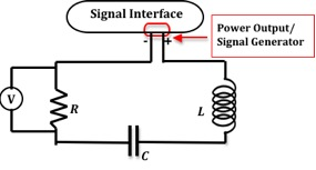
Figure 6: Schematic of circuit diagram

Insert the iron core into the center of the inductor. This increases the inductance of the coil. For the particular circuit board that you will use in this lab, the inductance of the coil (with the iron core inserted) is 33 mH.

The power amplifier will be used as the voltage source. Connect its output terminals to the resistor and capacitor as shown, using the banana plug patch cords.

Plug one voltage sensor DIN plug into analog channel A of the signal interface, and connect its leads across the 10-ohm resistor. The voltage measured at analog channel A will be used to calculate the current, I, which is related to the voltage

V_R

across the resistor. See Eq. (3).

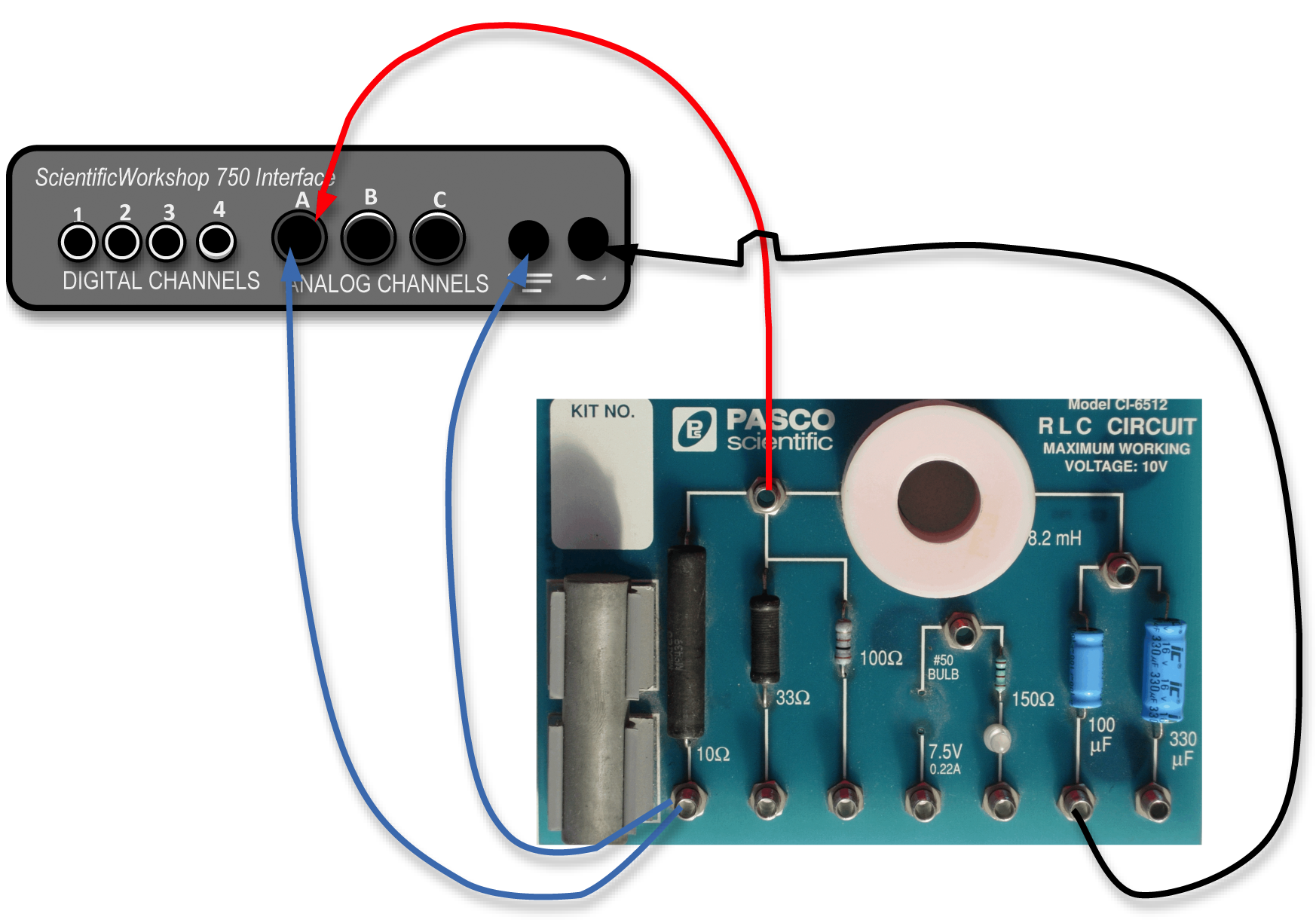
Figure 7: Details of connections

Checkpoint 1:
Ask your TA to check your circuit.

Turn on the computer and monitor, the signal interface, and the power amplifier.

Open the Capstone file associated with this lab, which starts the Capstone program. A screen similar to Fig. 8 is displayed.

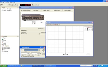
Figure 8: Opening screen in Capstone

Check that the signal generator is set to produce a sine wave having a frequency of 10 Hz and an amplitude of 5 volts.

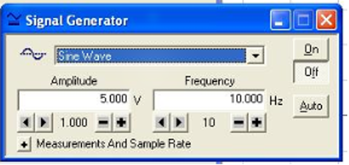
Figure 9: Signal generator settings

Record this as the voltage

V₀

on the worksheet.

Click ON, then click START to begin data acquisition.

To view the resonance, sweep through the frequencies by changing the settings in the signal generator window. You can do this by clicking the up and down arrows or by clicking on the number and typing in a new value. As you step through the frequency, notice that

V_R

increases as the frequency approaches the resonant frequency and then decreases as the frequency is increased beyond the resonant frequency. Also notice that the phase difference between the voltage output by the amplifier and

V_R

goes to zero at the resonant frequency.

Use the Show Data Coordinates tool to measure the voltages across the resistor

V_R

and the source

V₀.

Click the button and move to the point you want to measure. See Fig. 10 below.

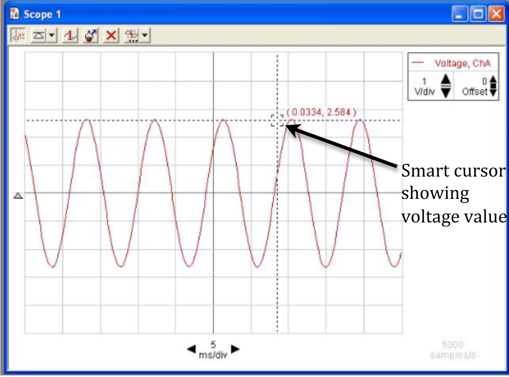
Figure 10: Screenshot showing the Show Data Coordinates button

Increase the frequency by 10 Hz. Record this frequency on the worksheet and repeat step 12.

Repeat steps 12 and 13 until 160 Hz is reached. As the frequency is increased, it may be necessary to adjust the sweep speed and the vertical scale to get a clear trace of the

V_R

on the screen.

Look at the data taken and determine approximately at what frequency resonance occurred by seeing where

V_R

was a maximum. Set the signal generator to this frequency and make fine adjustments in the frequency until the trace of the current is in phase with the voltage. The circuit is now being driven at the resonant frequency. Record this value on the worksheet.

Using the resonant frequency calculate the resonant angular frequency using

ω _res = 2πf_res.

Calculate the theoretical resonant frequency using Eq. (22) and the values of L, C, and R.

Compare the measured resonant frequency to this theoretical value by computing the percent error. See Appendix B. Do not quit Capstone.

Checkpoint 2:
Ask your TA to check your data and calculations.

Procedure B: Determining Phase Shift

Left click on the ''Voltage'' label on the left side of the score window, then choose Add Similar Measurement, then choose Output Voltage.

Set the frequency to 10 Hz and examine the wave forms. Fig. 11 shows a screenshot of both voltages.

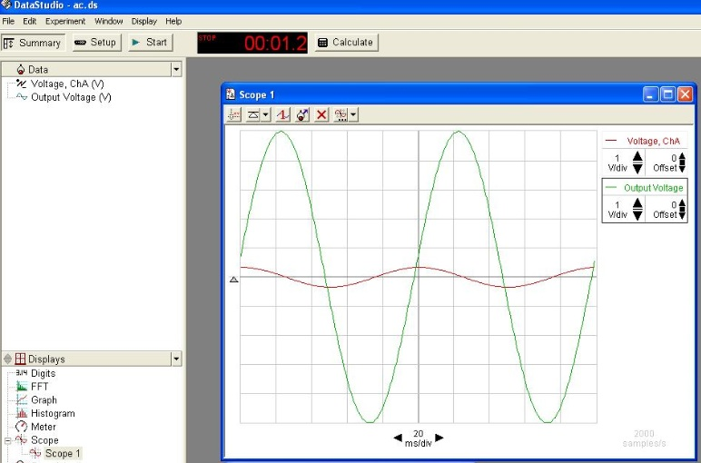
Figure 11: Screenshot showing the output voltage and the resistor voltage

Determine if the voltage peak across the resistor occurs before or after the output voltage peak. You may find it useful to take a very small time period of data and adjust the scale on the scope to look at the initial voltages.

If the time interval between a peak of

V₀

and a peak of

V_R

Δt,

then the magnitude of the phase difference is

φ = 2π (fΔt).

Repeat this to find the phase shift for a frequency of 160 Hz.

Checkpoint 3:
Ask your TA to check your data and calculations.