
Measurements of a Table
Objectives
-
•to practice the concepts of significant figures, the mean value, the standard deviation of the mean and the normal distribution by making multiple measurements of length and width of a table
-
•to estimate and measure the area of the laboratory table and reported with the correct number of significant figures and correct format
-
•to practice the propagation of errors by determining the uncertainty in the measurement of the area of the table
-
•to understand the difference between precision and accuracy
Equipment
- 20-cm wooden rod
- laboratory table
- measuring tape or 2-m metric ruler
- Graphical Analysis (GA) Software
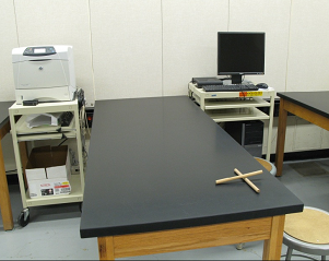
Figure 1
Introduction and Theory
Physics is largely a science of measurements. Experience has shown that no measurement is exact. All measurements have some degree of uncertainty due to the limits of instruments and the people using them. In science, it is critically important to specify that uncertainty, and include its reliable estimate in the final statement of the result of the measurement. Two concepts associated with measurements are accuracy and precision. The accuracy of the measurement refers to how close the measured value is to the true or accepted value. For example, if you used a balance to find the mass of a known standard 100.00 g mass, and you got a reading of 78.55 g, your measurement would not be very accurate. In general, the experimantal results are considered accurate if the percent discprepancy/difference is within 10-15%, depending on the experimental setup used to prove the theoretical concept. Precision is the degree of exactness or refinement of measurements. Precision has nothing to do with the true or accepted value of a measurement, so it is quite possible to be very precise and totally inaccurate. In many cases, when precision is high and accuracy is low, the fault can lie with the instrument. If a balance or a thermometer is not working correctly, they might consistently give a systematic error (inaccurate answers) resulting in high precision and low accuracy. In general, the experimental results are considered to be precise if the relative uncertainty is less than 5-10%, depending on the experimental setup used to prove the theoretical concept. One important distinction between accuracy and precision is that accuracy can be determined by only one measurement, while precision can only be determined with multiple measurements. A measurement can be accurate but not precise, precise but not accurate, neither, or both. For example, if an experiment contains a systematic error, then increasing the sample size generally increases precision, but it does not improve accuracy. Eliminating the systematic error improves accuracy, but it does not change precision. Commonly, the best estimate of the true value of the measured quantity x can be obtained by calculating the mean (average) value of some significant N number of measurements of that quantity repeated using the same equipment and procedures.( 1 )
x =
| N |
| ||
 | |||
| i = 1 |
( 2 )
σx =
= Δx,
| σx | ||
|

( 3 )
σx =
 |
|
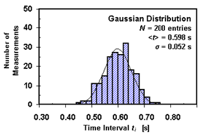
Figure 2: An example of a histogram and a normal distribution for the measurements of time
Error Propagation
The mean value of the physical quantity, as well as the standard deviation of the mean, can be evaluated after a relatively large number of independent similar measurements have been carried out. These calculated quantities in many cases serve as a basis for the calculation of other physical quantities of interest. In such situations, the uncertainties associated with the directly measured quantities affect the uncertainty in the quantity that is derived by calculations from those quantities. To estimate the uncertainty (error; standard/random error or standard deviation of the mean) in the final result, the error needs to be propagated. The rules of error propagation for the first approximation are the following, where f (function) is the derived physics quantity, Δf is an uncertainty in the derived quantity,x
and y
(variables) are the mean values of the quantities that are being measured, and Δx and Δy are uncertainties (standard deviation of the mean) in these mean values.
Rule 1: addition/subtraction: f(x, y) = x + y or f(x, y) = x − y
( 4 )
(Δf) = Δx + Δy
f(x, y) = xy or f(x, y) =
| x |
| y |
( 5 )
| Δf |
| f |
| Δ x |
| x |
| Δ y |
| y |
f(x, y) = xm
( 6 )
| Δf |
| f |
| Δx |
| x |
f(x, y) = Cx,
where C is a constant
( 7 )
(Δf) = CΔx
f(x, y) = Cxm yn,
where C is a constant
( 8 )
| Δf |
| f |
| Δx |
| x |
| Δy |
| y |
( 9 )
% discrepancy =
· 100%
 |
| (Ameasured − Aestimated) |
| Ameasured |
|
( 10 )
Rel. uncertainty =
· 100%
| ΔA |
| A |
Procedure
Please print the worksheet for this lab. You will need this sheet to record your data.
1
Open the Graphical Analysis (GA) program. The default file consists of a two-column table and a graph area. Double click on the first column name and change its label for the length along with the units - cm. In the same way, change the name and unit of the second column for width.
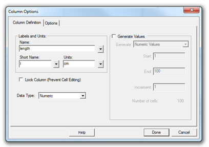
Figure 3
2
Measure the length of the laboratory table with the unmarked wooden rod provided on the table. To make measurements, use only one hand. Do not make any marks on the table with a pen or a finger. You need to have a total of 30 quick, seemingly nonchalant measurements of each dimension. Remember the length of one rod is 20 cm. Make the measurement in centimeters and estimate each measurement of length up to 1 cm. Report your measurements in cm in GA in the correponding column. (Do not worry about over- or underestimating the measured quantity; the mean value should be the most probable value for your measurements anyway.)
3
Make the length vs length graph in GA. Select data on the y-axis of the graph, and press the STAT button.
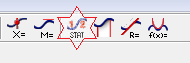
Figure 4
The statistical value including mean values and standard deviation will appear in the box. Record them in Table 1 provided on the Lab 1 worksheet.
4
Repeat step 2 and 3 to obtain the mean value of the width of the table as well as the standard deviation. Record those two values in Table 1 provided on the Lab 1 worksheet.
(Hint: Add a new graph window to make width vs width graph. From the pull-down INSERT menu, select Graph. Left clicking on the label of the axis will allow you to choose the data you want to plot on that axis.)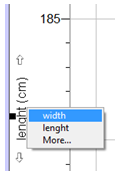
5
Measure the length and width of the table with measuring tape. (Ask your TA for the measuring tape). Record the length and the width of the table with the correct number of significant figures in Table 2 provided on the Lab 1 worksheet. Check with your TA that you record the measurement value with the correct number of significant figures. The uncertainy of the measurement equals the smallest division of the instrument.
6
Now we will check if the data of length that you collected with a 20-cm unmarked wooden rod resembles the normal bell-shape distribution. To present graphically the distribution of collected data, make a histogram. From the pull-down INSERT menu, select ADDITIONAL GRAPHS → HISTOGRAM. Change histogram features by double-clicking the histogram window. In the open histogram dialog window, you can select the Bin Size and the Bin Start. Play around with these settings to see how they affect the display.
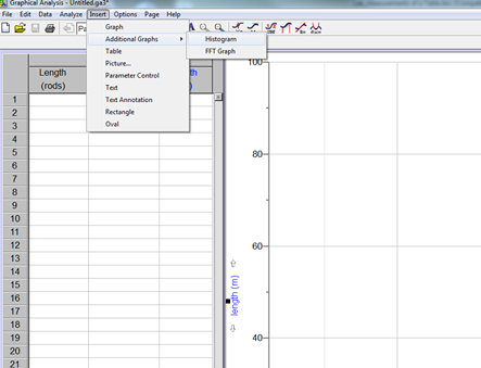
Figure 6
7
On the Histogram count, the number of measurements that falls within one standard deviation from the mean, and the number of measurements that falls within two standard deviations from the mean. Record both numbers on the Lab 1 worksheet.
8
Put all your experimental data that you collected in this lab from the Lab 1 worksheet into the Lab Report (not Inlab) part Data. The instant feedback identifies if your experimental data fits within the expected experimental range. If it does not, check if you collected these data using the correct method. Finally, explain the reasons for all major discrepancies in the discussion.
9
Re-size and rearrange the 3 graph windows (length vs length; width vs width; length histogram) to fit all of them on one page. Capture the screen and paste it into the MS Word document. Print it for your TA to sign it. Save this file for your future reference and upload it in the InLab. Be sure you can read all the data provided to you on the graphs.
10
Using your experimental data, you will need to find the estimated and measured area of the table with the uncertainties. To achieve the objectives of the lab, you will also find the percentage of data that fits within one and two standard deviations from the mean value of length to see if the collected data resembles normal distribution. Be sure to report all your results with the correct number of significant figures and in the correct format.
(Hint: First, remember to report only one significant figure in the uncertainty unless it equals one; in that case, report two significant figures. Secondly, report the mean value and its uncertainty to the same number of decimal places. The rules of handling significant figures can be also found in the document Basic Concepts of Error Analysis or the power point presentation Results and Uncertainties that is available under Lab Materials on Blackboard for your course.)
11
Complete the Lab Report on WebAssign. Be sure you save your entries as you work on the lab report. Be sure to submit your lab report by the due date posted on WebAssign.