
Linear Motion
Objectives
-
•to compare the relationship between position vs time and velocity vs time for different types of linear motion
-
•to learn to find the characteristics of linear motion from a position vs time graph and a velocity vs time graph
-
•to measure the value of gravitational acceleration g on Earth by the free fall method and compare it to the accepted value
Equipment
- battery powered constant velocity buggy
- masking tape
- cardboard
- PASCO motion sensor
- sail cart
- track
- small rubber object and whiffle ball
- stopwatch
- 30-m measuring tape
- picket fence with 5-cm band spacing
- wide photogate on stand
- floor mat
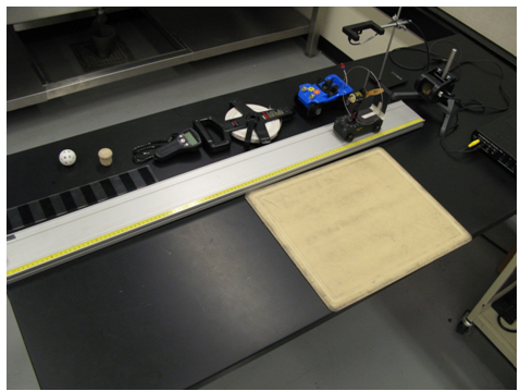
Figure 1
Introduction and theory
Kinematics is the area of physics that studies types of motion without specifying what caused it. The three major types of simple linear motion are constant velocity motion, uniformly accelerated linear motion, and free fall. The basic physics quantities used to describe the motion of an object are: position, distance, displacement, speed, velocity, and acceleration. The description is sufficient if one can specify the location of the object at all times. Position is simply the distance from an arbitrary chosen point called the point of reference. The point of reference is usually aligned with the origin on the coordinate axis. For one dimensional motion (or motion in a straight line), the position at any time can be specified by a single value, x or y, with units of distance. Positions to the right of the origin will be given a positive sign; positions to the left will be negative. Distance is the length of the path along with the object moved. For one dimensional motion in a constant direction, it is an absolute magnitude of the difference between final and initial position. Distance is always a positive value. The SI unit for distance is meter. The displacement, s, is a vector that points from an object's initial position toward its final position and has a magnitude equal to the shortest distance between the two positions. Unlike distance, displacement can be assigned a positive or negative sign depending on the direction of the object's motion. In the case of motion along a straight line, a displacement in the direction increasing position value will be assigned a positive value, and a displacement in the opposite direction will be negative. The SI unit for displacement is a meter. Speed is the rate at which distance is traveled. Speed is given by distance traveled divided by the elapsed time and is expressed in the SI units m/s. Speed indicates how fast the object is moving, but it does not include any reference to the direction of motion. Speed has always a positive value.( 1 )
speed =
| distance |
| elapsed time |
( 2 )
average velocity =
or vave =
.
| displacement |
| elapsed time |
| Δx |
| Δt |
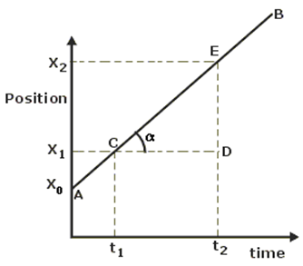
Figure 2: Position vs time plot
( 3 )
slope = velocity =
=
= tan α
| x2 − x1 |
| t2 − t1 |
| DE |
| CD |
( 4 )
x(t) = x0 + vt,
( 5 )
average acceleration =
or vave =
| change in velocity |
| elapsed time |
| v2 − v1 |
| t2 − t1 |
Kinematics Equations
Derived from the definitions of velocity and acceleration, there are three basic kinematic equations governing the motion with constant acceleration. To simplify our notation, we assume that the initial time t1 = 0 s. The position at any given instant of time, t, of an object moving with constant acceleration, a, having initial position x0 and initial velocity v0, can be found as( 6 )
x = x0 + v0t +
at2.
| 1 |
| 2 |
x = x0 + v0t +
at2.
| 1 |
| 2 |
( 7 )
v = v0 + at
( 8 )
v2 = v02 + 2a(x − x0).
Free Fall
If air resistance is negligible, the motion of the object caused by the gravitational force is known as free fall. A free-falling object experiences a uniformly accelerated motion until it reaches its terminal velocity. Everything on Earth experiences gravitational acceleration from the Earth. The acceleration of a freely falling object, g, is constant and equals approximately 9.81 m/s2 near the surface of the Earth. Since free fall motion is uniformly accelerated motion, the equations of kinematics that describe uniformly accelerated motion can be used. Consider the picture in Fig.3, below. An object at rest is released from a position of y above the floor.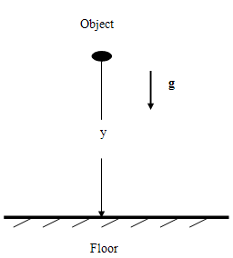
Figure 3: Free fall diagram
y(t) = y0 + v0t +
,
| gt2 |
| 2 |
( 9 )
y(t) = y0 + v0t +
,
| gt2 |
| 2 |
( 10 )
y(t) =
.
| gt2 |
| 2 |
Procedure
Please print the Lab 2 Worksheet. You will need this sheet to record your data.
Part 1. Cart moves toward the motion sensor at a constant speed.
1
Place the constant speed buggy at the opposite end of the track from the motion detector. Using masking tape, make a mark on the track 20 cm away from the motion sensor. Turn on and hold the buggy. Start the program and release the buggy. Stop the recording when the buggy reaches a 20 cm mark.
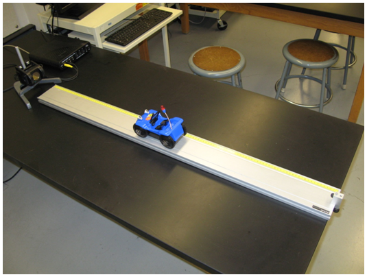
Figure 4
2
You should see on the screen the position vs time graph and velocity vs time graph of the buggy's run produced by the software. Use the Autofit function to resize the graphs.
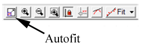
Figure 5
3
On the position vs time graph choose two points far apart from each other using the "Smart Tool".
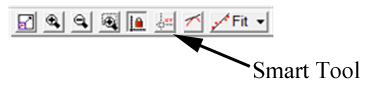
Figure 6
4
In Table 1 in the Lab 2 worksheet, clearly state the time values, t1 and t2, and the corresponding positions, x1 and x2. The data will be used to calculate the distance, displacement that the buggy travels as well as its average velocity and average speed.
5
In Table 2 in the Lab 2 worksheet, record the time and position of two consecutive points, chosen somewhere at the beginning of the buggy's movement. The data will be used to calculate the instantaneous velocity at that instant.
6
In Table 3 in the Lab 2 worksheet, record the time and position of two consecutive points, chosen somewhere at the end of the buggy's movement. The data will be used to calculate the instantaneous velocity at this instant.
7
On the position vs time graph, highlight (drag around with the computer cursor) the part of the plot corresponding to the buggy moving along the track with constant speed. Apply Linear Fit. (Hint: Select Linear Fit in the pull down Fit menu.)
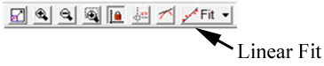
Figure 7
8
Record the slope and y-intercept for this graph in the Lab 2 worksheet. What physical quantities do the parameters of the Linear Fit represent?
9
Carefully highlight the part of the velocity vs time graph where the velocity looks mostly like a steady horizontal line, and apply Statistics to get the mean value of the velocity. (Hint: Select Statistics from the Σ pull down menu.)
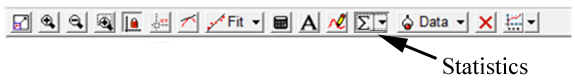
Figure 8
Record the mean value of the buggy's velocity in the Lab 2 worksheet.
10
Make a printscreen of the graphs with the data. Paste it and save it in the .doc format to upload it later in the InLab.
Part 2. Uniformly accelerated motion
1
Attach a piece of the cardboard to the side of the sail cart facing the motion detector. Place the sail cart 20 cm away from the motion detector and oriented so that it will move away from the motion detector. Turn on the fan and start the program. Stop recording the data when the cart reaches the other end of the track. Stop the cart.
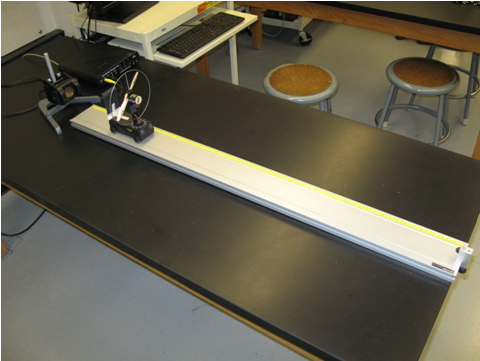
Figure 9
2
On the position vs time graph, highlight the curved part of the graph corresponding to the cart accelerating along the track. Fit the selected part of the data with a Quadratic Fit function.
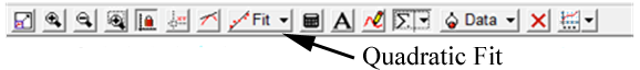
Figure 10
Record the values of the parameters in Table 4 in the Lab 2 worksheet. What physics quantity does each parameter represent?
3
Velocity is directly proportional to the time. Apply Linear Fit to the velocity vs time graph. Record the slope and y-intercept in Table 5. What physics quantity is the slope of this line? What physical quantity is the y-intercept of this line?
4
Make a printscreen of the graphs with the data. Paste it and save it in the .doc format to upload it later in the InLab.
Part 3. Free fall: A. Stairway
1
Drop a rubber object (provided) from the stairway of a building. Make sure that no one is directly below the object when it is dropped. Use a tape measure to determine the height y from which the object is released. Use the stopwatch to measure the time t it takes for the object to fall down to the ground. These measurements have to be repeated at least 10 times in order to get a reasonable value of t
along with the associated error.
Record measurements of the height and time in the Lab 2 worksheet. Assume the error in height is 2.0 cm.
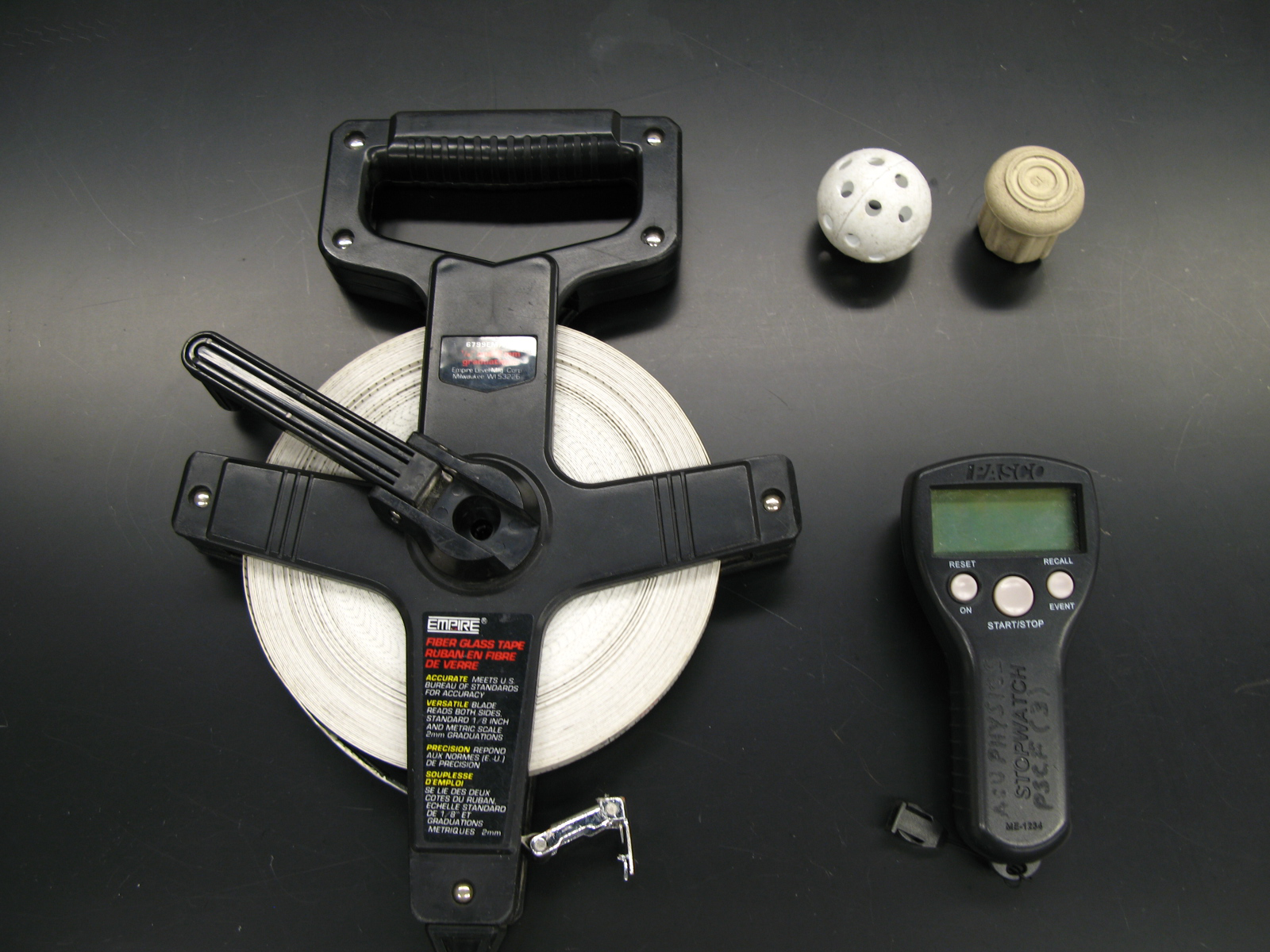
Figure 11
2
Repeat the same procedure for a whiffle ball. Record measurements of the height and time in the Lab 2 worksheet. Assume the error in height is 2.0 cm.
3
Enter the values of the measured time in GA and use statistics to find the mean value of time and its error for each object separately.
4
Make a printscreen of the graphs with the data. Paste it and save it in the .doc format to upload it later in the InLab.
5
Using these data, you will evaluate the value of gravitational acceleration g that each object has experienced, and its uncertainty.
Part 3. Free fall: B. Photogate
1
Turn on the interface and open the pre-set experiment file: Labs/PHY 113/PreSet upFiles/Free Fall.
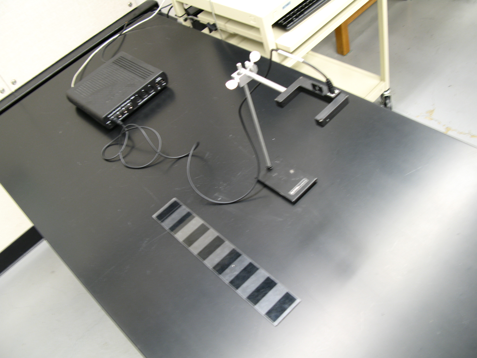
Figure 12
2
Position the stand with a photogate at the edge of the lab table in such a way that you can safely drop the long picket fence all the way through. Bring the rubber or foam pad directly underneath the photogate onto the floor to cushion the landing of the picket fence. Try to catch the picket fence after it passes through the photogate.
3
Press the "Start" button and carefully drop the picket fence through the photogate. The software stops collecting the data automatically after 5 seconds. Apply the linear fit to your velocity data displayed on the graph to get the acceleration of the falling picket fence. Repeat this procedure 5 times.
4
In GA, create a new manual column. (Hint: Data→New Manual Column.) Remember to name it and choose an appropriate unit.
Enter the values of the measured acceleration in Graphical Analaysis and use statistics to state the final value of your experimental g along with its error.
Enter all your data from the Lab 2 worksheet into the InLab. Remember to upload graphs that were produced in the lab in the .doc format.
In your lab report, you will need to find the characteristics of the buggy's motion (distance, displacement, average speed, average velocity, instantaneous velocity), and calculate the free fall acceleration and its uncertainty. Write equations of the buggy's motion and the sail cart's motion and compare them.