
The Pendulum
Objectives
-
•to verify Galileo's observations that the period of a pendulum is independent of the mass and angular amplitude (for small angles)
-
•to determine how the period of a pendulum depends upon the length of the string
-
•to calculate the experimental mass of Earth
Equipment
- set of 6 identical washers that will act as the simple pendulum
- support stand with a photogate connected to the Science Workshop interface
- meter stick
- protractor
Introduction and Theory
A simple pendulum consists of a point mass and a string. The point mass is suspended at one end of the string and the other end of the string is held fixed. The motion of a pendulum takes place in a vertical plane as illustrated in fig. 1, where the angle θ is measured from the vertical line to the string. The gravitational force exerted upon the mass m can be decomposed into two perpendicular components. The sum of the forces in the direction along the string is( 1 )
Ts − mg cos θ = mar,
ar = v2/r
is the radial acceleration. In the other direction, the sum of the forces is
( 2 )
−mg sin θ = mat,
−g sin θ.
This acceleration is tangent to the path of the pendulum at every point.
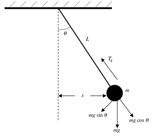
Figure 1: The force diagram for a pendulum.
sin θ ≈ tan θ ≈ x/L,
and eqn. 2−mg sin θ = mat,
becomes
( 3 )
Fnet = −mg
= −
x.
| x |
| L |
 |
| mg |
| L |
 |
Fnet = −mg
= −
x.
is the equation for simple harmonic motion and from this the period of the pendulum can be determined to be
| x |
| L |
|
| mg |
| L |
|
( 4 )
T = 2π
.
 |
|
( 5 )
T = 2π
1 +
sin2
+
sin4
+ ...
.
|
|
|
| 1 |
| 4 |
| θ |
| 2 |
| 9 |
| 64 |
| θ |
| 2 |
|
T = 2π
1 +
sin2
+
sin4
+ ...
.
|
|
|
| 1 |
| 4 |
| θ |
| 2 |
| 9 |
| 64 |
| θ |
| 2 |
|
( 6 )
| ΔT |
| T |
| 1 |
| 4 |
| θ |
| 2 |
| 9 |
| 64 |
| θ |
| 2 |
Procedure
Please print the worksheet for this lab. You will need this sheet to record your data.
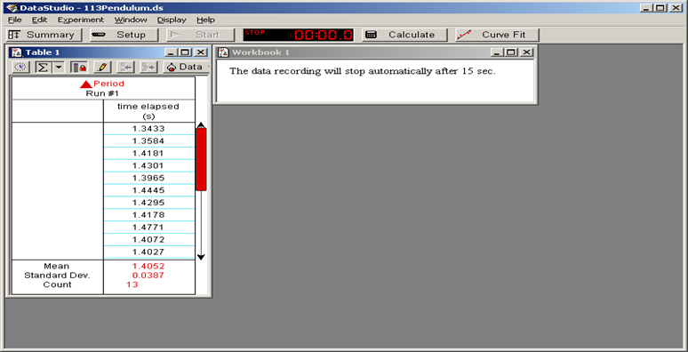
Figure 2: A sample of the DataStudio® file for the pendulum exercise.
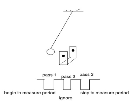
Figure 3
Be aware that the photogate can get confused if the string crosses the beam or if the beam passes through the opening in a washer. Use masking tape to close the opening in a washer. Always keep an eye on the pendulum while it is swinging so that it does not drift into a collision with the delicate and expensive photogate.
Experiment I: Measure the period of oscillations for pendulum bobs of different masses while keeping the length of the pendulum and amplitude fixed.
Allow the mass to swing back and forth a couple of times before you start making measurements to let the pendulum "settle". To start the data acquisition, press the "Start" button on the tool bar menu. Use small amplitudes (angles) of about 5°.1
Put one washer at the end of the string. In Graphical Analysis, create columns to record the mean times (in seconds) and the number of the washers. All of the washers have the same mass, so the numbers of washers is proportional to the mass of the pendulum bob. START the timer in DataStudio®. It will stop automatically in 15 s. Record the mean value shown in DataStudio® of the period in the GA.
2
Continue changing the mass of the pendulum by adding one washer at a time. Measure the period of oscillations for each mass. Keep recording the mean value of the period and the number of the washers in GA.
3
In Graphical Analysis, make a graph of the pendulum period (the mean value) vs. the mass (the number of washers). All of the washers have the same mass, so the numbers of washers are proportional to the mass of the pendulum bob.
4
Record the slope and its uncertainty of the period vs mass graph in the Lab 7 worksheet.
Experiment II: Measure the period of oscillations for pendulum bobs at different amplitudes while keeping length and mass fixed.
1
In Graphical Analysis, create columns to record the mean value of the period and the starting amplitudes (angles). Place two washers on the string. START the timer in DataStudio®. It will stop automatically in 15 s. Record the mean value of the period in the GA.
2
Repeat measurements of the period of oscillations for angles 5°, 10°, 15°, 20°, 30°, and 40°.
3
Discuss the relationship between period and amplitude in the discussion section. Address in your discussion if the period stayed constant for all the angles.
Experiment III: Measure the period of oscillations for pendulum bobs while varying length.
Keep the initial angle (e.g. 10°) and mass (two-washers) constant. The length of a simple pendulum is the distance from the pivot point to the center of mass of the pendulum bob.1
Measure the period of oscillations for 6 different lengths of the pendulum.
2
Enter your measured values of the period T (the mean value) and corresponding length L into GA. Create a new column for the value of T2 (DATA-NEW CALCULATED COLUMN). Plot T2 vs. L and apply linear fit from the Analyze pull down menu. The slope of this graph and its error will allow you to determine the acceleration due to gravity (g) and the error. Record the slope of the graph and its error in the Lab 7 worksheet.
From Equation 4 :
T = 2π
.
|
|
( 7a )
T = 2π
 |
|
( 7b )
T2 = 4π2
| L |
| g |
( 7c )
T2 =
· L = slope · L
| 4π2 |
| g |
( 7d )
slope =
.
| 4π2 |
| g |
3
The slope and its uncertainty are calculated by the computer. Use the rules for error propagation to determine the uncertainty in g. The relative error for the calculated gravitational acceleration can be found as:
( 8 )
| Δg |
| g |
| Δslope |
| slope |
4
Report your results of the gravitational acceleration and its error in the result section.
Calculating the mass of Earth
Since the factor of g occurs in the period of a pendulum, it is possible to use the measurements taken above to determine the mass of the Earth. The acceleration due to gravity near the surface of the Earth is defined as( 9 )
g =
.
| GME |
| rE2 |
T = 2π
.
|
|
( 10 )
T = 2π
.
|
|