Impulse, Momentum, and Energy – Procedure

Objective

In this lab, you will verify the Impulse-Momentum Theorem by investigating the collision of a moving cart with a fixed spring. You will also use the Work-Energy Theorem to evaluate the energy losses during the collision.

Equipment

Track
Force sensor with spring bumper
Cart with low friction wheels
Photogate
Meterstick

Procedure

Please print the worksheet for this lab. You will need this sheet to record your data.

Experimental Setup

The experimental setup consists of a long, inclined track to which a force sensor with a spring is attached. See Figure 2. A cart will be released from the high side of the track and will roll down the incline, collide with the spring, and then roll back up the incline. A photogate will be placed just in front of the spring to measure the speed of the cart just before and just after the collision.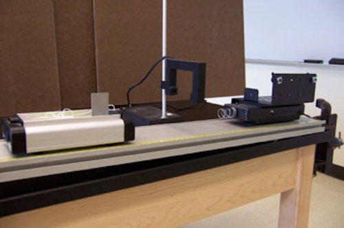

A force sensor is positioned at the bottom of an inclined track with its spring facing up the track. A photogate is positioned a short distance up the track from the spring. Above the photogate on the incline is a cart, which has a square, metal flag attached to the top of the cart's lower end.

Figure 2: A force sensor with spring bumper

The cart moves down the track, collides with the spring, and goes back up the track. The force sensor will record the force of this collision at equally spaced time intervals. Plotting this force information, you will be able to determine impulse from the area under the force vs. time curve. From the initial and final speeds of the cart recorded by the photogate measurements, you can determine the change in momentum of the cart. You can then compare the impulse to the change in momentum to validate the impulse-momentum theorem.

Energy

During this process, some of the cart's energy will be lost due to the action of non-conservative forces. You will be able to see this in two ways. First, the initial and final speeds recorded by the photogate will not be equal, indicating that energy is lost due to the action of non-conservative forces during the collision. According to equation 7 in the Impulse, Momentum, and Energy – Concepts document, the energy lost during the collision is equal to the work done by these non-conservative forces.

( 8 )

ΔE_collision = W_NC^collision

Secondly, after the collision, the cart will return to a point on the inclined track that is lower than the point from which it was initially released. This shows a net loss of energy over the entire trip. Some of this energy is lost during the collision as shown in equation 8, and some is lost to other non-conservative forces acting while the cart travels down and up the ramp. Therefore, the total energy lost during the entire trip will be equal to the work

W_NC^collision

done by non-conservative forces during the collision, plus the work

W_NC^traveling

done by the other non-conservative forces acting while the cart travels along the track. In other words,

( 9 )

ΔE_total = W_NC^collision + W_NC^traveling.

Let's now try to determine these energy losses in terms of quantities that can be determined experimentally. We will first focus on the energy loss that occurs over the entire trip,

ΔE_total.

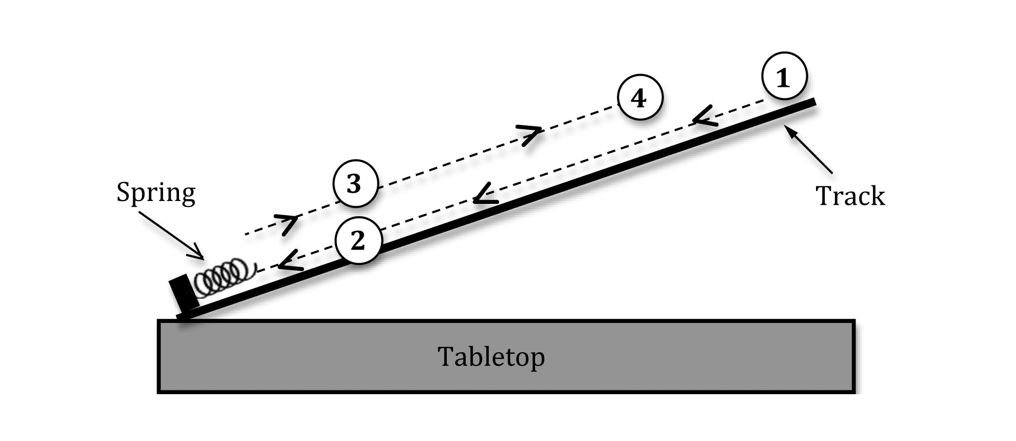
A rectangle labeled Tabletop forms an acute angle with a line labeled Track. An object labeled Spring is attached to another rectangle connected to the lower end of the Track such that the Spring is parallel to the Track. A thin dashed line parallel to the Track points down the Track from a point at the top of the Track labeled Point one to the Spring passing through a point near the Spring labeled Point two. Another thin dashed line parallel to the Track points up the track from the Spring to a point a short distance from the top of the Track labeled Point four passing through a point near the Spring labeled Point three.

Figure 3: Diagram of the path of the cart

Figure 3 is a diagram of the trip taken by the cart. The cart is released from location Point one

, travels down the ramp and first passes through the photogate at location Point two

just before the collision. This is represented by the thin dashed line with arrows pointing down the track. The cart then bounces off the spring and passes back through the photogate at location Point three

just after the collision. This is represented by the thin dashed line with arrows pointing up the track. Note that locations Point two

and

are actually the same positions on the track. Finally, the cart returns to location Point four

, which is lower on the track than the initial starting location Point one

. The two dashed lines are displaced from each other for clarity. Combining equations 5 and 7 in the Impulse, Momentum, and Energy – Concepts document, we get

( 10 )

ΔE_total = ΔK_total + ΔU_total

where

ΔK_total = K₄ − K₁

and

ΔU_total = U₄ − U₁.

Since the cart is released from rest and returns to rest,

K₄ = K₁ = 0

and

( 11 )

ΔE_total = U₄ − U₁.

If we focus on determining the energy loss just in the collision itself (i.e., from location Point two

on the way down back to location Point three

on the way up), we have

( 12 )

ΔE_collision = ΔK_collision + ΔU_collision

where

ΔK_collision = K₃ − K₂

and

ΔU_collision = U₃ − U₂.

Since the cart is at the same height each time it passes through the photogate,

U₃ = U₂,

and we get

( 13 )

ΔE_collision = K₃ − K₂.

Equations 11 and 13 can be used to determine the total energy loss and the energy loss just in the collision, respectively. Then, this information can be combined with equations 4 and 5 in the Impulse, Momentum, and Energy – Concepts document to determine the work,

W_NC^collision,

done by non-conservative forces during the collision, and the work,

W_NC^traveling,

done by other non-conservative forces while the cart travels along the track.

Initial Set-up

The equipment consists of a straight track, a cart with low friction wheels, a force sensor with a spring bumper, and a photogate. A computer acquires, stores, and displays the data collected by the photogate and force sensor.

Weigh and record the mass of the cart on the worksheet.

Measure the width of the flag on the cart and record it on the worksheet.

Make sure the track is set up so that the yellow, ruled strip is facing you, and make the side of the track flush with the edge of the table.

Elevate the starting end of the track about 4 to 5 centimeters so that the cart can roll toward the spring bumper.

Move the track so that the end with the force sensor is firmly against the stop.

Set the photogate so that the flag clears it 1 to 2 centimeters before the cart hits the spring bumper.

Calibrating the Force Sensor

Open the appropriate Capstone file associated with this lab. The force probe will automatically be routed to analog channel A and the photogate will automatically be routed to digital channel 1.

Click the Timer Setup window. See Figure 4.

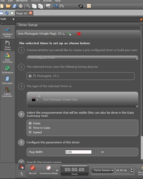
Figure 4: Capstone window showing input for flag width

Enter your flag width.

Click the Calibration button on the left side menu.

Choose Force as the sensor to calibrate, then Two Standards (2 points), the click next. See Figure 5.

The calibrate sensors window in Capstone has a group of settings at the top titled Sensor, Measurement, Unit. The first box in this group is set to Force Sensor, the next box is set to Force (N), and the option Calibrate all similar measurements simultaneously is not selected. Beneath these settings are boxes that display the Slope and Offset of the Previous Calibration and the Present Sensor Measurement. Beneath these boxes is an option titled Calibration Type with radio button 2 Point (Adjust Slope and Offset) selected. Next there are input boxes for the Standard Value and Sensor Value for Calibration Point 1 and Calibration Point 2 with both calibration point groups having a Read From Sensor button. These are followed by a group of boxes that display the Slope and Offset of the New Calibration.

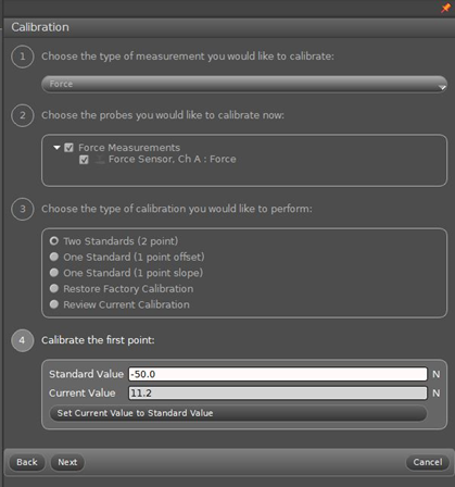
Figure 5: Calibrate sensors

Remove the force sensor from the track by loosening the bolts on the side.

After the Calibrate Sensors window opens, go through the following steps.

a
Hang the 500 g (4.95 N) mass from the spring (the force sensor should be in one hand with the mass hanging below the sensor).
b
Input –4.9 N in the Standard Value box. Notice the (–) sign. Click Set Current Value to Standard Value, then click Next.
c
Remove the mass.
d
Flip the sensor so that the spring is pointing up toward the ceiling. Steady the 500 g (4.95 N) mass on the spring.
e
Input +4.9 N in the second Standard Value box. Notice the (+) sign. Click Set Current Value to Standard Value, then click Next.
f
Click Finish to complete the calibration process.
g
Click on the right edge of the calibration window and slide it to the left to make the table and graph visible.

Return the force sensor to the track and tighten. Make sure the force sensor, clamp, and track all remain in place when the car slides down the track and hits them.

Now you are ready to begin the lab!

Data Acquisition

Select a starting point about 60 cm from the end of the spring bumper. Record this on the worksheet as the starting position.

Note:

This is the distance up the ramp from the uncompressed spring.

Use the meterstick to measure the vertical distance from the bottom of the tabletop to the top edge of the track at the starting position. Record this in the worksheet as the starting position height.

Place the cart so that the end with the flag is towards the spring bumper and the front end is lined up with the starting position.

Click the Record button to start the data acquisition program and then release the cart, being careful not to push it either up or down the track. The cart should go through the photogate once on its way down and once on its way up the track for a total of two passes. Now click the Stop button. Practice Steps 3 and 4 a few times before performing the experiment. You should be able to get the cart to return to roughly the same place each time it is released, and you should have a nice, smooth force vs. time curve like the one shown in Figure 6.

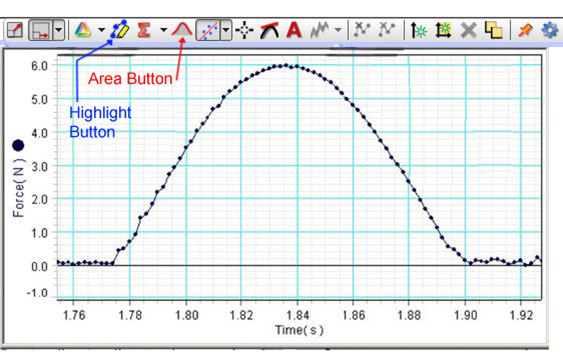
A graph of force (N) versus time (s) composed of many individual points connected by line segments. The graph forms a relatively smooth curve that is approximately zero and nearly horizontal for a short time interval, increases to a maximum and decreases back down to approximately zero forming a parabolic arc in the middle of the graph, and remains approximately zero and nearly horizontal for the short remainder of the graph. Near the top of the graph window is a toolbar with buttons. Arrows are drawn pointing to the fourth button from the left labeling it Magnifying tool and pointing to the twelfth button from the left labeling it Summation button.

Figure 6: Screenshot showing plot of spring force versus time

Observe the position of the back end of the cart (the end that was originally at the starting position) when it temporarily stops at its maximum height. Record this on the worksheet as the stopping position.

Measure the vertical distance from the bottom of the tabletop to the top edge of the track at the stopping position. Record this in Table 1 in the worksheet.

Record the values of the initial and final speeds of the cart in Table 1.

Do not delete the data set. You will need it for future analysis.

Checkpoint 1:
Ask your TA to check your data from the first run before proceeding.

Repeat this procedure two more times with the exact same starting position.

Record the stopping position, track height, and the initial and final cart speeds each time in Table 1. At the end of this procedure, you should have three nice graphs of force vs. time, three sets of initial and final cart speeds, and three sets of stopping positions and track heights.

Checkpoint 2:
Ask your TA to check your data from the last two runs before proceeding.

Procedure A: Impulse

For each of the trials, do the following.

a
In the Capstone window, grab the numbers on the time axis and slide them to the right to spread out the data on the graph, then grab the graph (click on the inside of the graph) and move it left or right so the relevant portion of the graph fills a reasonable part of the graph window.
b
Click on the Highlight button (See Figure 6).
c
With just this portion of your graph highlighted, click the Area button.
d
This will automatically calculate the area under the highlighted portion of your graph. Enter this value of the area in Table 2 in the worksheet.
e
For one of the graphs, calculate the area by the trapezoid method to compare with the value obtained from the computer software. Construct rectangles between two data points with a height equal to the average of the two data points. Then the area is the sum of the areas of these rectangles.

Use the photogate speeds to compute the magnitude of the change in momentum of the cart for each trial and record these in Table 2 in the worksheet.

Calculate and record the average values of the area and change in momentum.

Compare the average area with the average change in momentum by computing the percent difference. See Appendix B.

Checkpoint 3:
Ask your TA to check your impulse calculations.

Procedure B: Energy

For each trial, use the initial and final speeds recorded by the photogate to calculate the energy loss during the collision. Record these in Table 3 on the worksheet.

For each trial, use the starting height and stopping height to compute the total energy loss for the entire trip. Record these values in Table 3.

Compute and record the average values of

ΔE_collision

and

ΔE_total.

Use these average values to determine the percentage of the total energy loss that occurred during the collision.

Use the average energy losses to determine the amount of work done by non-conservative forces during the collision as well as the amount of work done by other non-conservative forces during the rest of the cart's trip.

Caution 4:
Ask your TA to check your energy loss calculations.