
Conservation of Mechanical Energy – Procedure
Objective
In this experiment, you will roll a ball down a ramp situated above a table as in Figure 1.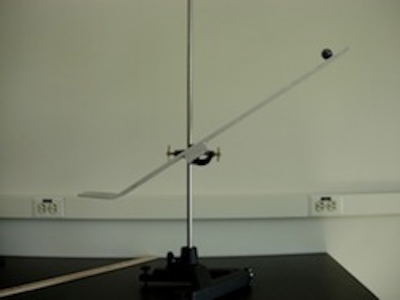
Figure 1
-
1Kinematics, treating the ball as a point mass in free fall
-
2Energy, looking at conservation of the ball's energy
Equipment
- Metal track and stand
- Marble
- Meterstick
- Carbon paper
- White paper
- Tape
Background
The objective of this experiment is to determine if conservation of mechanical energy can predict the velocity of a rolling sphere after rolling down a ramp. You will test your hypothesis by placing the sphere at various heights and measuring the velocity at the end of the ramp. You will compare the measured velocity with the predicted velocity using conservation of mechanical energy. If we let the sphere roll down a ramp, its vertical height will decrease while its translational and rotational velocity will increase. Potential energy is lost and kinetic energy is gained. Assuming that the sphere rolls without slipping and there is no friction or air drag, the loss of potential energy will equal the gain in kinetic energy. Based on conservation of mechanical energy, if the sphere is placed at heighth1,
as shown in Figure 2, you can show that the final speed v2
at the end of the ramp is

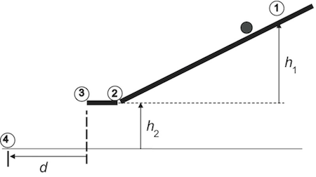
Figure 2
v2
of the sphere at point  at the bottom of the inclined portion of the ramp if we know the initial height
 h1.
In the experiment you will measure the translational speed of the sphere at the bottom of the ramp and compare it to the speed predicted by the conservation of mechanical energy. If these two (experimental and predicted) values of the translational speed agree to within experimental uncertainties, you can say that you have verified conservation of mechanical energy.
Experimental Design
Let us consider several ways in which the translational speed of a small sphere can be measured.-
1Use a police radar speed gun: A radar gun or speed gun is a small Doppler radar unit used to detect the speed of objects, especially trucks and automobiles for the purpose of regulating traffic, as well as pitched baseballs, runners or other moving objects in sports. It relies on the Doppler Effect applied to a radar beam to measure the speed of objects at which it is pointed. Radar guns may be hand-held or vehicle-mounted; see "Radar gun" or "Police RADAR".
- A radar speed gun measures the instantaneous speed of the sphere. As the sphere rolls down the ramp, its speed changes. It would be difficult to read the radar gun at the precise moment when the small sphere reaches the bottom of the ramp.
-
2Use an ultra sonic motion detector: The sonic motion detector transmits a burst of ultrasonic pulses. The ultrasonic pulses reflect off a target and return to the face of the sensor. The target indicator flashes when the transducer detects an echo. The sensor measures the time between the trigger rising edge and the echo rising edge. It uses this time and the speed of sound to calculate the distance to the object. To determine velocity, it uses consecutive position measurements to calculate the rate of change of position. See, for example, PASCO or Vernier.
- In general, a sonic motion detector used in a physics lab can only detect objects no smaller than a baseball. Measuring the speed of a small steel marble would be unreliable.
-
3Use a photogate: A photogate monitors the motion of objects passing through its gate, counting events as the object breaks the infrared beam. If the size of the object is known, by measuring the time an object blocks the gate, you can determine the velocity. See, for example, Vernier or PASCO.
- The size of the infrared beam from a photogate is not small compared to the diameter of the sphere. Thus you could not make an accurate determination of the length passing through the infrared beam.
-
4Use kinematics: Once the sphere leaves the ramp, it is under free fall. By measuring the vertical and horizontal components of the sphere's displacement after it leaves the ramp, you can determine the sphere's speed at the end of the ramp. Measuring the horizontal and vertical displacements of the sphere does not involve the use of motion detectors or photogates and is straight forward. You will use this method for the experiment.
Finding the speed using kinematics
The ramp has a short horizontal section from point to point  . We assume that the sphere's speed down the ramp does not change when it travels on the short horizontal section between point and point . Once the sphere leaves the ramp, there is no force acting on it to change its horizontal velocity (assuming there is no air resistance). Gravity pulls the sphere down the instant it leaves the ramp. We will consider the equations of motion for the vertical and horizontal motions of the sphere.
The vertical distance
. We assume that the sphere's speed down the ramp does not change when it travels on the short horizontal section between point and point . Once the sphere leaves the ramp, there is no force acting on it to change its horizontal velocity (assuming there is no air resistance). Gravity pulls the sphere down the instant it leaves the ramp. We will consider the equations of motion for the vertical and horizontal motions of the sphere.
The vertical distance h2
that the sphere falls in time ΔT
is given by
where g
= 9.81 m/s2 is the acceleration due to gravity. The initial vertical component of the velocity of the sphere as it leaves the ramp is zero.
The horizontal distance d
the sphere moves from the end of the ramp to the point where it touches the table is given by
Using equation 2 and equation 3, we can show that
Procedure
Please print the worksheet for this lab. You will need this sheet to record your data.
Kinematics
The first method will apply the principles of uniformly accelerated motion to treat the ball as a projectile. Measuring d and h2 as illustrated in Figure 2 will be enough to calculate the velocity of the ball at the time it leaves the ramp. As a reminder, the uniformly accelerated motion equations are reproduced below. For more details on this method, refer to the Concepts document.( 5 )
| vx | = | vx,0 + axt | vy | = | vy,0 + ayt | |||||
| x | = | x0 + vx,0t +
| y | = | y0 + vy,0t +
| |||||
| vx2 | = | vx,02 + 2ax(x − x0) | vy2 | = | vy,02 + 2ay(y − y0) |
1
Arrange the track and stand as illustrated in Figures 1, 2, and 3. Make sure the bottom part of the track is flat and that the ball won't roll off the sides on its way down.
2
Hold the ball steady at a point on the track and record the vertical distance from the table to the
ball. (Hint: Should you measure to the top, middle, or bottom of the ball?) As illustrated in Figure 3, the height, h1, will be the difference between this distance and h2, the distance from the table to the flat part of the track.
3
Release the ball and record where it lands. One method of doing this is to use the supplied
carbon paper. If you use carbon paper, put a blank piece of paper down where the ball will
land, then the carbon paper black-side-down on it. The ball's impact will make a mark on the
paper. If you use the paper, make sure to hold or tape it still so it doesn't slide when the ball impacts.
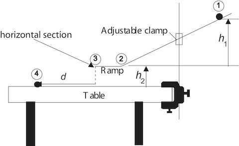
Figure 3
The horizontal distance from the edge of the ramp to the impact point will be d as illustrated in Figure 3. The vertical distance from the ramp to the table surface will be h2.
4
In order to improve the accuracy of the data, you will perform this measurement two more times
using the same starting height (that is, the same h1), finding the average value for d over the trials. Then for further accuracy, you will repeat the experiment with different starting locations, performing three trials for each different h1.
5
Finally, use the kinematics equations and the collected data to determine the velocity of the ball at
the instant it left the ramp.
Energy
Next, you will calculate the speed of the ball as it leaves the ramp again, this time using conservation of energy methods. During the ball's roll down the ramp, we will assume that it is rolling without slipping. This would mean that friction, while present, is not doing any work. If we also ignore the very small contribution due to air resistance, the conclusion is that the ball has no nonconservative force doing work on it and thus its mechanical energy is conserved. As a reminder, here are the expressions for various types of mechanical energy. Note that for a solid sphere,I =
MR2.
| 2 |
| 5 |
1
Using the data you collected in the Kinematics section, calculate the velocity at the bottom of the
ramp for each starting height. Use the starting position (at the top of h1) and the end of the ramp as your initial and final points. Should these calculations yield the same results as the kinematics calculations?
Conclusion
1
What are some of the sources of uncertainty in this lab that could have contributed to a discrepancy in the two data sets or to one or both of the calculations being too high or low? Specify which calculation method each source of uncertainty would contribute to, and whether it would tend to make the calculation too low or too high.
2
Considering all the sources of uncertainty you identified above, which method of calculation do you feel is likely to give a more accurate result? Consider how many sources of uncertainty each method might have and the magnitude of those uncertainties in your conclusion.