
Lab 4 - Charge and Discharge of a Capacitor
Introduction
Capacitors are devices that can store electric charge and energy. Capacitors have several uses, such as filters in DC power supplies and as energy storage banks for pulsed lasers. Capacitors pass AC current, but not DC current, so they are used to block the DC component of a signal so that the AC component can be measured. Plasma physics makes use of the energy storing ability of capacitors. In plasma physics short pulses of energy at extremely high voltages and currents are frequently needed. A capacitor can be slowly charged to the necessary voltage and then discharged quickly to provide the energy needed. It is even possible to charge several capacitors to a certain voltage and then discharge them in such a way as to get more voltage (but not more energy) out of the system than was put in. This experiment features an RC circuit, which is one of the simplest circuits that uses a capacitor. You will study this circuit and ways to change its effective capacitance by combining capacitors in series and parallel arrangements.Discussion of Principles
A capacitor consists of two conductors separated by a small distance. When the conductors are connected to a charging device (for example, a battery), charge is transferred from one conductor to the other until the difference in potential between the conductors due to their equal but opposite charge becomes equal to the potential difference between the terminals of the charging device. The amount of charge stored on either conductor is directly proportional to the voltage, and the constant of proportionality is known as the capacitance. This is written algebraically as( 1 )
Q = CΔV.
ΔV
in volts (V), and the capacitance C in units of farads (F). Capacitors are physical devices; capacitance is a property of devices.
Charging and Discharging
In a simple RC circuit, a resistor and a capacitor are connected in series with a battery and a switch. See Fig. 1.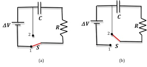
Figure 1: A simple RC circuit
( 2 )
ΔV −
− R
= 0.
| Q |
| C |
| dQ |
| dt |
ΔV −
− R
= 0.
is
| Q |
| C |
| dQ |
| dt |
( 3 )
Q = Qf
1 − e(−t / RC)
 |
 |
Qf
represents the final charge on the capacitor that accumulates after an infinite length of time, R is the circuit resistance, and C is the capacitance of the capacitor. From this expression you can see that charge builds up exponentially during the charging process. See Fig. 2(a).
When the switch is moved to position 2, for the circuit shown in Fig. 1(b), Kirchhoff's loop equation is now given by
( 4 )
| Q |
| C |
| dQ |
| dt |
| Q |
| C |
| dQ |
| dt |
( 5 )
Q = Q0e(−t / RC)
Q0
represents the initial charge on the capacitor at the beginning of the discharge, i.e., at t = 0.
You can see from this expression that the charge decays exponentially when the capacitor discharges, and that it takes an infinite amount of time to fully discharge. See Fig. 2(b).
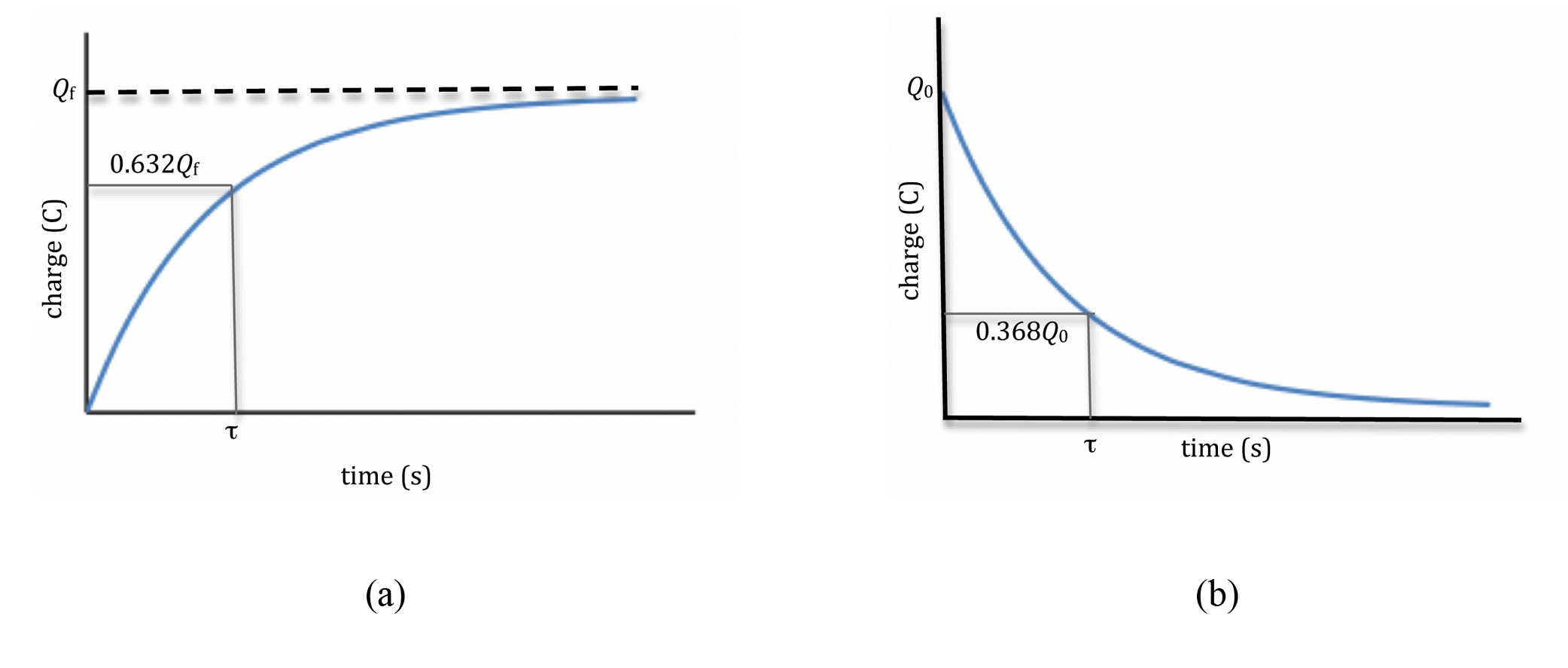
Figure 2: Change versus time graphs
Time Constant τ
The productRC
(having units of time) has a special significance; it is called the time constant of the circuit. The time constant is the amount of time required for the charge on a charging capacitor to rise to 63% of its final value. In other words, when t = RC,
( 6 )
Q = Qf
1 − e−1
 |
 |
( 7 )
1 − e−1 = 0.632.
(e−1 = 0.368)
of its initial value.
We can use the definition (I = dQ/dt)
of current through the resistor and Eq. (3) Q = Qf
1 − e(−t / RC)
and Eq. (5) |
|
Q = Q0e(−t / RC)
to get an expression for the current during the charging and discharging processes.
( 8 )
charging: I = +I0e−t/RC
( 9 )
discharging: I = −I0e−t/RC
I0 =
in Eq. (8)| ΔV0 |
| R |
charging: I = +I0e−t/RC
and Eq. (9)discharging: I = −I0e−t/RC
is the maximum current in the circuit at time t = 0.
Then the potential difference across the resistor will be given by the following.
( 10 )
charging: ΔV = + ΔVfe−t/RC
( 11 )
discharging: ΔV = − ΔV0e−t/RC
ΔV
in Eq. (9)discharging: I = −I0e−t/RC
and Eq. (11)discharging: ΔV = − ΔV0e−t/RC
are negative. This voltage as a function of time is shown in Fig. 3.

Figure 3: Voltage across the resistor as a function of time
Q = C ΔV,
Eq. (3)Q = Qf
1 − e(−t / RC)
and Eq. (5) |
|
Q = Q0e(−t / RC)
that describe the charging and discharging of a capacitor can be rewritten in terms of the voltage. Merely divide both equations by C,
and the relationships become the following.
( 12 )
charging: ΔV = ΔVf
1 − e(−t/RC)
|
|
( 13 )
discharging: ΔV = ΔV0e(−t/RC)
Q = Qf
1 − e(−t / RC)
and Eq. 5 |
|
Q = Q0e(−t / RC)
. The graph of the voltage across the capacitor versus time is shown in Fig. 4 below.
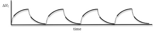
Figure 4: Voltage across the capacitor as a function of time
charging: ΔV = ΔVf
1 − e(−t/RC)
we get
|
|
( 14 )
| ΔVf − ΔV |
| ΔVf |
( 15 )
−ln
=
.
 |
| ΔVf − ΔV |
| ΔVf |
 |
| t |
| RC |
−ln((ΔVf − ΔV)/ΔVf)
versus time will produce a straight line graph with a slope of 1/RC. Similarly, for the discharging process, Eq. 13discharging: ΔV = ΔV0e(−t/RC)
can be rewritten to get
( 16 )
| ΔV |
| ΔV0 |
( 17 )
−ln
=
.
|
| ΔV |
| ΔV0 |
|
| t |
| RC |
−ln(ΔV)/ΔV0)
versus time will produce a straight line graph with a slope of 1/RC.
Using a Square Wave to Simulate the Role of a Switch
In this experiment, rather than using a switch, we will be using a signal generator that can generate periodic wave forms of varying shapes, like a sine wave, triangular wave, and square wave. Both the frequencies and amplitudes of the wave forms can also be adjusted. Here we will use the signal generator to produce a time-varying voltage, with a square wave form, across the capacitor similar to the one shown in Fig. 5.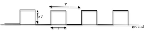
Figure 5: A square wave with period Τ
T = 2t
is the period of the square wave. During the first half of the cycle, when the voltage is positive, it is similar to the switch being in position 1. During the second half of the cycle, when the voltage is zero, it is the same as the switch being in position 2. So the square wave, which is a DC voltage that is turned on and off periodically, serves as both battery and switch in the setup in Fig. 1
The signal generator allows this switching to be done repeatedly, and it is possible to optimize the data collection by adjusting the frequency of the repetition. This frequency will depend on the time constant of the RC circuit.
When the time t is larger than the time constant τ of the RC circuit, the capacitor will have enough time to charge and discharge, and the voltage across the capacitor will be as shown in Fig. 4.
Objective
In this experiment a (computer-emulated) oscilloscope will be used to monitor the potential difference, and thus, indirectly, the charge on a capacitor. The voltage measurements will be used in two different ways to compute the time constant of the circuit. Finally, capacitors will be connected in parallel to examine their equivalent circuit capacitance.Equipment
- PASCO circuit board
- Signal interface with power output
- Connecting wires
- Capstone software
Procedure
Please print the worksheet for this lab. You will need this sheet to record your data.
Setting Up the RC Circuit
The RLC circuit board that you will be using consists of three resistors and two capacitors among other elements. See Fig. 6 below. In theory you can, therefore, have different combinations of resistors and capacitors. In this experiment you will use the 33-Ω and 100-Ω resistors and the two capacitors.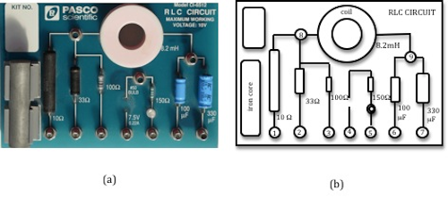
Figure 6: RLC circuit board
1
Connect the far right output terminal of the signal interface to the 33-Ω resistor at point 2.
2
To bypass the inductor, connect a wire from point 8 to point 9.
3
Connect point 6 to the second output terminal of the signal interface to complete the circuit.
4
Connect the voltage probe into analog channel A.
5
To measure the voltage across the capacitor, connect the black lead of the voltage probe to point 6 and the red lead to point 9.
Make sure that the ground of the interface (the "–" lead) is connected to the same side of the capacitor as the ground of the signal generator (power output).
Your circuit connection should look like that in Fig. 7.
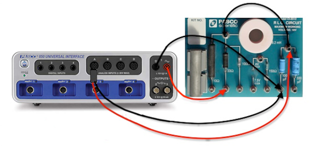
Figure 7: Circuit diagram
Checkpoint 1:
Ask your TA to check your circuit connections.
Ask your TA to check your circuit connections.
Procedure A: Time Constant of the Circuit
We will use the computer to emulate the oscilloscope in this experiment.6
Open the Capstone file associated with this lab. A screen similar to Fig. 8 is displayed.
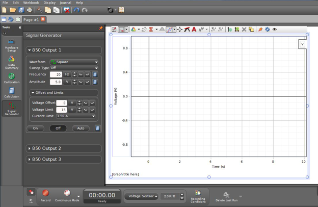
Figure 8: Opening Screen of Capstone File
7
Set the signal generator to produce a positive square wave by choosing the positive square wave in the signal generator window as shown in Fig. 9 below.
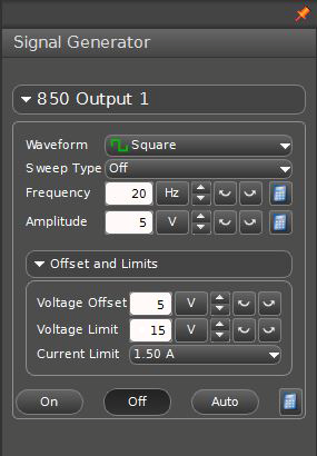
Figure 9: Signal generator window
8
If not already set when the Capstone file opens, set the signal generator to produce a square wave of 5-V amplitude at a frequency of 20 Hz, and set the voltage offset to 5 V.
9
Turn on the signal generator by clicking ON in the signal generator window.
10
To monitor the signal, click the START button in the main window. It will be necessary to adjust the time and voltage scales to produce a signal trace like that shown in Fig. 10. This will allow you to observe how the voltage on the capacitor varies as a function of time. To do this, set the cursor on any value along the axis you wish to zoom on, and move the cursor left-right or up-down as needed. When properly zoomed, you will have only one wavelength in the graph display like the trace in Fig. 10.
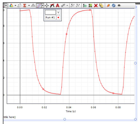
Figure 10: Signal trace
If at any time you want to delete a recorded data set, click on the Delete Last Run button below the graph.
11
Select the Show Coordinates button from the buttons above the graph. See Fig. 11.
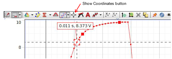
Figure 11: Show Coordinates
When show coordinates is active, a read-out of the voltage and time is displayed wherever you drag it, as in Fig. 11. Using this tool, determine and record the starting time (i.e., when the trace started upward from 0 volts) on the worksheet.
12
Calculate 63.2% of the maximum voltage, ΔVf,
(which should be 5 V), the setting on the amplitude of the signal generator.
Using Show Coordinates, determine and record the starting time (i.e., when the trace started upward from 0 volts) on the worksheet.
13
From these two time values, determine and record the time required for the signal to go from ΔV = 0 to ΔV = 0.632ΔVf.
This is your experimental value for RC.
14
On the worksheet, fill in the accepted values for the resistance and the capacitance, which are printed on the circuit board.
15
Compute the experimental value of the capacitance using your experimental value for RC and the accepted value of R. Record this on the worksheet.
16
Compute the percent error using the two values for the capacitance. See Appendix B.
Checkpoint 2:
Ask your TA to check your data and calculations before proceeding.
Ask your TA to check your data and calculations before proceeding.
Procedure B: Calculation of Capacitance by Graphical Methods
17
Record the maximum voltage on the worksheet.
18
From the recorded data, find the times at which ΔV = 1, 2, 3, and 4 volts on the rising part of the curve using the smart tool. Record this information in Data Table 1 on the worksheet.
Note: You might need to zoom in a lot to get the precision you need when using the smart tool.
19
Perform the necessary calculations to complete Data Table 1.
20
Using Excel, plot −ln((ΔVf − ΔV) / ΔVf)
versus time. See Appendix G.
21
Use the trendline option in Excel to draw the best fit line to your data, determine the slope of the line and record this value on the worksheet. See Appendix H.
22
From the value of the slope, determine the time constant and the capacitance. Record these values on the worksheet.
23
Compute the percent error between this value of the capacitance and the accepted value.
Checkpoint 3:
Ask your TA to check your data, graph, and calculations before proceeding.
Ask your TA to check your data, graph, and calculations before proceeding.
Procedure C: Measuring Effective Capacitance
Capacitance adds directly when capacitors are connected in parallel and inversely when connected in series. This is opposite of the rule for resistors. For capacitors in parallel, the effective capacitance is given by( 18 )
Ceff = C1 + C2 + C3 + . . .
( 19 )
| 1 |
| Ceff |
| 1 |
| C1 |
| 1 |
| C2 |
| 1 |
| C3 |
24
Connect the second capacitor (330 μF) in parallel with the capacitor used in procedure A by connecting a wire from point 6 to point 7.
25
Switch the resistor to the 10-Ω resistor by moving the connection from point 2 to point 1.
26
Record another data set by clicking START in the main window.
Once you have recorded the second data set, you might want to display only that data on the graph and remove data set 1. To do this, delete the first run (see the note in Step 10).
You will be looking at just one wavelength in the graph display.
27
For this part of the experiment, you will consider the discharging portion of the curve.
Now the initial voltage ΔV0
will be the highest value of the peak before the graph starts to fall off. Record this value on the worksheet.
28
From the recorded data, find the times at which ΔV = 1, 2, 3, and 4 volts on the falling part of the curve using the smart tool. (Note: You might need to zoom in a lot to get the precision you need when using the smart tool). Record this information in Data Table 2 on the worksheet.
29
Perform the necessary calculations to complete Data Table 2.
30
Using Excel, plot −ln(ΔV) / ΔV0)
versus time.
31
Use the trendline option in Excel to draw the best fit line to your data, determine the slope of the line and record this value on the worksheet.
32
From the value of the slope determine the time constant and record this value on the worksheet.
33
Compute Ceff,
the effective capacitance of the parallel combination, using the accepted value for R.
34
Compare this experimental value with that you obtained from Eq. 18Ceff = C1 + C2 + C3 + . . .
and the accepted values of the capacitance by computing the percent error between the two values.
Checkpoint 4:
Ask your TA to check your data and calculations before proceeding.
Ask your TA to check your data and calculations before proceeding.