
Electric Fields and Potentials
Introduction
Physicists use the concept of a field to explain the interaction of particles or bodies through space, i.e., the "action-at-a-distance" force between two bodies that are not in physical contact. For example, the earth modifies the surrounding space such that any object with mass, such as the moon, is attracted. We have seen previously in our study of the "Universal Law of Gravitation" that the gravitational field gets weaker as you go farther away from the source but never completely disappears. An electron similarly modifies the space around it in such a way that other particles with like charge are repelled, while particles with the opposite charge are attracted. Like the gravitational field, the electric field gets weaker with distance from the source but is never completely gone. Any charge placed in an electric field will experience a force, as will any mass placed in a gravitational field. Just as mass in a gravitational field has some potential energy, so does a charge in an electric field.Discussion of Principles
Electric Field
A charged body experiences a force, F, whenever it is placed in an electric field, E. The vector relationship between the force and the electric field is given by The magnitude of the force divided by the magnitude of the charge, q, on the body is numerically equal to the magnitude of the electric field. From Eq. (1), we see that the direction of the electric field vector at any given point is the same as the direction of the force that the field exerts on a positive test charge located at that point. A positive test charge will be repelled by a positive charge and attracted by a negative charge. Therefore, electric field lines start on positive charges and end on negative charges. The number of lines starting from a positive charge or ending on a negative charge is proportional to the magnitude of the charge. The electric field at any point is tangential to the electric field lines. The magnitude E of the electric field strength is proportional to the number of electric field lines per unit area perpendicular to the lines. A positive charge placed in an electric field will tend to move in the direction of the electric field lines and a negative charge will tend to move opposite to the direction of the electric field lines.Work, Potential Energy, and Electrostatic Potential
Work is done in moving a charged body through an electric field. The amount of work, W, done depends on the electric field, the magnitude of the charge and the displacement, d, that the charge makes through the field. When the displacement is so small that the electric field can be assumed uniform in the region through which the charge moves, the work, W, is given by the dot product of the force and displacement vectors. The negative of the work done by the electric force is defined as the change in electric potential energy, U, of the body. Put another way, it is the difference in the potential energies ΔU associated with the starting and ending positions. The electrostatic potential, V, is defined as the electric potential energy of the body divided by its charge:V = U/q
. Hence, in terms of electrostatic potential, the work done by the electric field is
where ΔV = Vfinal − Vinitial
is the potential difference.
The magnitude of the electric field can also be determined from Eqs. (3) and (5)
where θ is the angle between the field and displacement vectors.
When a charged particle moves in an electric field, if its electric potential energy decreases, its kinetic energy will increase. In other words, the total energy is conserved.
A positive charge placed in an electric field will tend to move in the direction of the field. The work done by the electric field in this case will be positive as the field and the displacement vectors are in the same direction and the dot product of the two vectors will be positive as shown in Figure 1(a). Note that the velocity vector indicates the direction of the displacement vector for the charge.

Figure 1: Motion of charges in an electric field
−W = ΔU = (Ufinal − Uinitial)
, we see that the change in electric potential energy will be negative in this case.
It will, therefore, lose electric potential energy and gain kinetic energy. This tells us that electric potential decreases in the direction of the electric field lines. A positive charge, if free to move in an electric field, will move from a high potential point to a low potential point.
Now consider a negative charge placed in an electric field as shown in Figure 1(b). It will tend to move in a direction opposite to the electric field and accelerate as it does so. The work done by the electric field will be
Again, note that the work done by the electric field is positive and the negative charge will lose electric potential energy and gain kinetic energy as it moves against the field. A negative charge, if free to move in an electric field, will move from a low potential point to a high potential point.
To move a positive charge against the electric field, work has to be done by you or a force external to the field. The charge is forced to move from a low potential point to a high potential point and the work done by the external force is negative. The reverse will be true for a negative charge.
As in the case of the gravitational field, the zero point of the electric potential is chosen arbitrarily. In general, the zero point is at infinity; however, often in circuits, the zero point for the potential is the ground or a conductor that is directly connected to the ground.
Equipotential Lines and Electric Field Lines
Consider the field due to a single point charge. A point in this space near the source of the field (i.e., near the point charge), and another point far from the source of the field are at different potentials. This is true even if no charges reside at the two points. In Fig. 2, points A and B are at different potentials due to the electric field of the positive charge.
Figure 2: Electric potential at different points in a field
−W = ΔU = (Ufinal − Uinitial)
that no work is done in moving a charge along an "equipotential" (i.e., an equipotential line or surface). Eq. (4) also tells us that no work is done when the displacement and the field are perpendicular to one another.
Therefore, the electric field vectors must be perpendicular to the equipotentials.

Figure 3: Electric field lines and equipotential lines
Mapping of the Electric Field
We employ a special conducting paper (not too conducting and not too insulating) and a voltmeter. Some shapes have been drawn on the paper, and to these we will connect a power supply. Because the paper is conducting, a current can flow between the electrodes. By Ohm's law, the current flows along the electric field. Thus, if we can measure either the current or the electric field, we can determine the other. With our equipment, we cannot directly measure the electric field; however, what we can do is measure voltage differences using the voltmeter setting on the multimeter. From these voltage differences we can learn about the electric field lines because the voltage difference between two points is a measure of the integrated electric field between the electrodes (see Eq. (6)E =
).
If the electric field is along the path between the leads, then | ΔV |
| d cos θ |
|ΔV|
is a maximum; if the electric field is normal to this path, then |ΔV| = 0.
Thus, when the voltmeter probes are separated by a fixed distance, the direction of maximum effect gives the direction of the electric field. The electric field points from high to low electrical potential (voltage). Recall that on the earth, the gravitational field points from high to low gravitational potential.
As noted above, the electric field lines are perpendicular to surfaces called equipotential surfaces. In two dimensions, these are lines. Along an equipotential, the electric field is a minimum—that is, it is zero. A voltmeter will yield zero voltage difference between two points that are on the same equipotential line. See Figure 4.

Figure 4
Apparatus
- DC power supply
- Multimeter
- Graphite-coated paper (with conducting designs) mounted on frames
- Two-lead holder
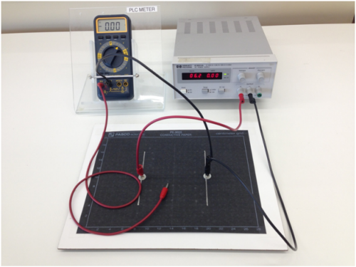
Figure 5: Apparatus
Procedure
Please print the worksheet for this lab. You will need this sheet to record your data.
Setting Up the Experiment
The graphite sheets provided have equally spaced division marks imprinted on them. The division marks may be used as reference when transferring data collected from the graphite sheets to a template that you will be supplied later in the lab. The graphite sheets also have various shapes (configurations) drawn on the surface with conducting nickel ink (similar to Figure 6). Graphite paper has been chosen for two reasons. First, the graphite paper has an electrical resistance that is much less than the voltmeter, so that the voltmeter will not draw much current. Second, it has a large enough electrical resistance that it does not draw more current than the power supply can provide.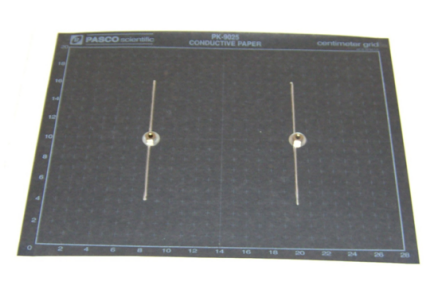
Figure 6: Parallel plate configuration
1
Set the multimeter dial to a resistance setting, and connect the two banana to banana leads to the jacks on the multimeter such that resistance may be measured.
With the end of the meter leads, measure the electrical resistance of the graphite paper for the distance of two division marks. Now place the meter leads on the conducting lines (also about two divisions apart) and measure the electrical resistance of the conducting line(s). What are the two values and are they different?
2
Why can't ordinary paper be used? Why can't a copper sheet be used?
Equipotentials for a Parallel Plate Configuration
1
Turn off the multimeter and set its dial such that the multimeter may be used to measure at least six volts. Insert a black (banana to banana) lead in the COM (short for common) jack of the multimeter and a red (banana to banana) lead in the V jack of the multimeter.
Turn on the multimeter. If you hear a buzz coming from the multimeter, turn it off immediately. You have probably put the red or black lead into the wrong jack or your dial is set to measure the wrong quantity. A correctly configured multimeter will display the volt unit on the LCD screen.
2
Locate the power supply on your lab table but do not connect it to the circuit yet.
Press the On/Off power button to the On position. Next, press the Range button to the "in" position (this sets the power supply to the 0-35 V/0-0.85 A range).
Rotate the Voltage and Current ADJUST knobs fully counterclockwise. Then set the maximum output current for this experiment by pressing the CC Set button, and while holding it down, rotate the current ADJUST knob clockwise until the AMPS display reads 0.50. Release the CC Set button.
Caution:
Do not move the Current setting knob after this adjustment is done (unless given instructions in the lab).
Do not move the Current setting knob after this adjustment is done (unless given instructions in the lab).
The Voltage ADJUST knob will be used to increase the voltage output as needed for the experiment. Keep the Voltage knob counterclockwise for now.
3
Connect the power supply output to the jacks of the graphite sheet that has two parallel conducting lines on it.
This geometry represents a two-dimensional version of a parallel plate capacitor. Turn the Voltage knob clockwise until the meter on the supply reads 6 V. With the multimeter set to measure voltage, you will measure the voltage difference between various points on each of the sheets.
Since current can't leave the conducting paper except at the two places connected to the power supply, when you make measurements close to the edge of the paper, you will find that the field will be oriented parallel to the paper's edge.
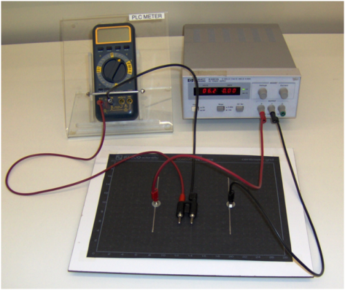
Figure 7: Two lead probes for measuring the direction of the E-fields
4
Using the multimeter (see Figure 5), measure the voltage difference between the two jacks on the graphite sheet. (It should read six volts.)
5
Equipotential surfaces are surfaces for which the voltage is the same. Determine the equipotential surface corresponding to 0.5 V and continue, in half-volt increments, until about 10 equipotential lines are found.
Record the positions of the x and y coordinates on the graphite sheets for each equipotential surface you wish to map. You should find at least 5 points on each surface you are mapping. Record these x, y values in an Excel spreadsheet.
Caution:
Be careful to not drag the multimeter probes over the surface of the conducting paper since this will damage the paper surface. Lift and press the probes against the paper at changing position increments until the equipotential you are searching for is located.
Be careful to not drag the multimeter probes over the surface of the conducting paper since this will damage the paper surface. Lift and press the probes against the paper at changing position increments until the equipotential you are searching for is located.
6
Once you have recorded the positions of these 10 equipotential surfaces in your spreadsheet, you can now use the scatter plot feature of Excel to map these surfaces. You can make the scatter plot for all of your equipotentials by placing the x coordinate of each measurement in column 1 and the associated y measurements for each surface in a different column for each of the values of the potential measured. Making the scatter plot this way results in each of the equipotential surfaces having a different symbol in the plot making it easy to connect-the-dots and sketch the equipotential surfaces. Copy your scatter plot from Excel into a MicroSoft Paint window. Using the Paint tools available, sketch the equipotentials in black and then draw in the E-field lines in red. (Save this sketch and upload to WebAssign.)
7
Connect the ends of the leads of the multimeter to the two-lead holder (see Figure 7), which makes the leads a fixed distance apart. Placing and orienting the leads of the holder on the graphite sheet surface to read the maximum voltage on the multimeter will show the direction of the electric field. Determine the direction of the field and indicate the direction on your sketch from step 6. Summarize your results.
Checkpoint:
Have your TA check your potential map for this configuration before uploading your picture and moving to the next step.
Have your TA check your potential map for this configuration before uploading your picture and moving to the next step.
Equipotentials for a Dipole Configuration
1
Turn off the power supply and then connect the leads of the power supply to another graphite paper configuration. (Now use the conducting paper configuration with the two circular electrodes painted onto them.)
Now turn the power supply back on, to 6 V.
2
Choose one of the jacks as a reference point for this portion of the experiment. Write down which one, so there is no confusion later.
3
Measure the potential difference between the two jacks. If it differs much from 6 V, see your instructor.
4
Using the same technique from mapping of the parallel plate configuration above, record the x, y
locations of at least 5 points on 10 different equipotential surfaces spaced by about 0.5 V for the dipole configuration. Enter this data into a new spreadsheet and then make a scatter plot of the potential surfaces as done above. (Note: You should repeat the process that you used in the previous section to map these surfaces.)
Once you have entered the equipotentials, you can now sketch the E-field lines corresponding to these potential surfaces using the rules governing these lines described in the lab write up.
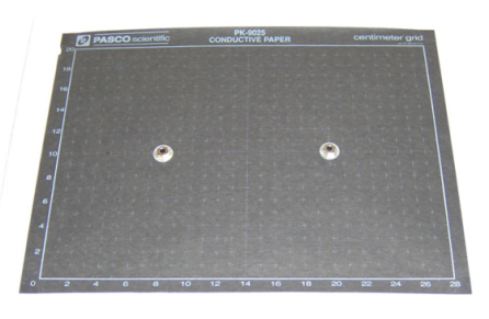
Figure 8: Dipole configuration
5
Using the two-lead holder, find the direction of the field lines. Summarize your results.
6
Now examine the equipotential lines at the edge of the graphite paper. Current cannot leave the graphite paper at the edge, so it flows parallel to the paper at the edge. Since the electric field lines are along the direction of current flow, at the edge of the paper the electric field lines should be along the edge. Check this with the electric field probe. Determine how the equipotential lines hit the edge of the paper. Summarize your results.
Checkpoint:
Once again have your TA check your potential map for this configuration before uploading your picture and moving to the next step.
Once again have your TA check your potential map for this configuration before uploading your picture and moving to the next step.
Equipotentials for the Surface and Point Configuration
1
Turn off the power supply and then connect the leads of the power supply to the "surface with a point" graphite paper configuration. Now turn the power supply back on (6 volts output).
2
Measure the potential difference between the two jacks. If it differs much from 6 V, see your instructor.
3
Using the same technique from mapping of the parallel plate configuration above, record the x, y
locations of at least 5 points on 10 different equipotential surfaces spaced by about 0.5 V for this new configuration. Enter this data into a spreadsheet and then make a scatter plot of the potential surfaces as done above. (Once again, use the procedure from the previous mapping exercises to find the equipotential surfaces for this configuration.)
Once you have entered the equipotentials, you can now sketch the E-field lines corresponding to these potential surfaces using the rules governing these lines described in lab write up.
4
Within the central region of this configuration, using the two-lead holder, find the direction of the field lines and summarize your results.
Checkpoint:
Once again have your TA check your potential map for this configuration before uploading your picture.
Once again have your TA check your potential map for this configuration before uploading your picture.