
Magnetic Fields
Introduction
This experiment concerns magnetic forces and fields. You will examine magnetic field lines and forces qualitatively, and measure field strengths using a Hall probe. A magnaprobe will also be used. The magnaprobe has a small swiveling magnet (north pole is labeled). Its mounting is fragile, so be gentle. The magnaprobe dipole axis will align parallel to a field, the north pole pointing in the direction of B. Also, all permanent magnets can be demagnetized by physical shock, so please do not drop them.The Hall Effect
The Hall effect relies upon magnetic forces experienced by charges carrying a current. The case is illustrated in the figure below. A current flows to the right, and a magnetic field, B, points into the page (see figure below). The magnetic force,I × B,
gives an upward force on the charge carriers, with the signs illustrated for negatively-charged electron charge carriers.
If the voltage leads (V+ and V–) experience a very high resistance (such as your 10 MΩ multimeter), almost no current can flow through them, and some of the charge carriers will collect at the upper edge of the Hall bar as shown in the figure. This leads to the observed Hall voltage,
as is shown in many texts (n is the carrier density, q is the charge, and t is the thickness). This voltage, proportional to B, can be used to measure B if the set of constants | I |
| nqt |
(EHall = VH/d).
An offset voltage added to VH is usually found, due to accidental offsets in the voltage leads, which are often spot-welded to the small sample. Offset leads will pick up the electric field given by Ohm's law, shown in the inset in Figure 1. This is why the probe must be zeroed in your experiment.
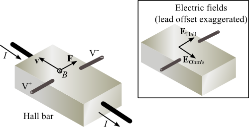
Figure 1
1/n,
where n is the charge-carrier density, Hall sensors use semiconductors in which n is small in order to obtain a large effect. In the case of your probe, the bar is gallium arsenide (GaAs). The Hall bar is tiny, hidden inside the tip of the probe, and it is oriented so that fields in line with the length of the probe have maximum effect. You will be able to verify that turning the probe 180° reverses the sign of the effect. Inside the box, there are two current leads that carry a 5-mA constant current, and two wires carrying the Hall voltage. The box also contains the source for the 5-mA current, and an amplifier circuit which magnifies the Hall voltage (by a factor of 10 or 100) so that it can be read by the multimeter. The output voltage is proportional to the magnetic field, aside from the zero adjustment, and the calibration is indicated on the Hall-sensor box.
Theory
The magnetic field, B, is a vector field, like the electric field. Field lines can be used to graphically indicate the direction of B, and the density of lines is proportional to the magnitude of B. Field lines are closed loops, always encircling currents, as in Figure 2. The closed-loop behavior holds for permanent magnets too, although it is not so obvious since the return paths are hidden inside.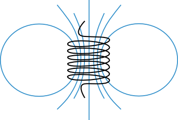
Figure 2
μ0 = 4π × 10−7 T · m · A−1.
Starting with Equation (2) we can find the fields due to complete loops of wire, for instance on the axis of an N-turn circular loop of radius, R,
This field points along the axis, in the right-hand thumb direction when the fingers are pointed along the current direction. The derivation is in most texts.
Current loops behave as dipoles. A loop of area, A, has a dipole moment, µ = IA,
where A points normal to the loop and in the direction given by the right-hand thumb if the fingers point along the current direction. For dipoles, B drops as 1/r3,
at large r. We see this specifically for the circular loop since the field in Equation (3) becomes | μ0NIR2 |
| (2x3) |
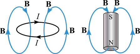
Figure 3
Apparatus
- 0-40 volt power supply
- Multimeter
- Hall probe box
- Circular coil (11 cm dia)
- Meterstick
- Masking tape
- Magnaprobe
- Cylindrical magnet
- Horseshoe magnet and keeper
- Compass
- Aluminum block (1 cm thick)
- Steel sheet (galvanized)
- Plastic block (1 cm thick)
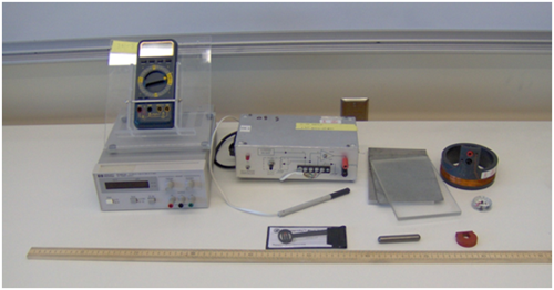
Figure 4
Procedure
Please print the worksheet for this lab. You will need this sheet to record your data.
Field Lines Due to a Permanent Magnet
Field lines indicate the field direction: arrows of the B vector are along the field lines everywhere.Caution:
Remember, the magnaprobe and magnets are both rather delicate.
Remember, the magnaprobe and magnets are both rather delicate.
1
First, use the magnaprobe to examine the field near the cylindrical ("cow") magnet. Do not hold the magnaprobe too close to the cow magnet. Strong magnetic fields will damage the magnaprobe. The small dipole in the magnaprobe makes an arrow pointing along the B field everywhere. Examine the 3-D nature of the field by looping the magnaprobe in different directions. Convince yourself that the field near each pole points toward or away from the pole.
2
Make a field map. Tape (or hold) both ends of the magnet near the top of a sheet of paper (see Figure 5). Place the page flat on your bench. Keep other magnets well away while mapping lines. Trace the magnet position on the paper, and mark the end having the north pole. Use the magnaprobe to find the field direction in one spot, and draw a small arrow there, with the arrow point toward the probe-needle north. Go in the arrow direction to a spot nearby, and find the field direction there. Repeating this, generate a string of arrows that traces out a field line. Map about four lines this way. Carefully remove the tape when finished. Your group should sketch this out on the field-line mapping template using Paint. You will upload this sketch.
You may use the small compass in place of the magnaprobe for this part, if preferred; the arrow tip should be at the "north-seeking" tip of the compass needle.
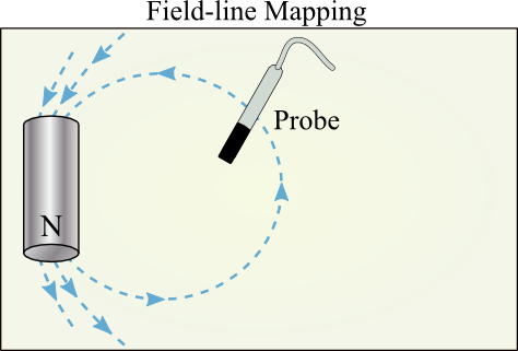
Figure 5
Using the Hall Probe
1
The Filter switch on the Hall probe box should be "on" for all of your measurements.
Set the digital multimeter to one of its Voltage ranges, and connect the Hall probe box output jacks to the digital multimeter. The leads plug into the common and Volts jack on the multimeter. The multimeter beeps if the leads are plugged into the wrong sockets.
If you cannot get the multimeter to stop beeping, turn off the meter and ask your instructor for assistance.
2
Use the magnaprobe to find the Earth's field direction. The Earth field points north, but somewhat inclined to the ground, rather than horizontal. Lightly tapping the magnaprobe will allow it to register the direction. Try this a couple of times to make sure you have a true direction. (Sometimes the magnaprobe tip comes off the bearing, and will not rotate easily. You might try the compass, which will give the horizontal direction of the field, but not the inclination angle.)
3
Turn on the Hall probe box if it is not already on. With the filter "on," turn the Hall probe box Range switch to x100. Set the digital multimeter to the 200 mV scale, and DC. Hold the Hall probe so that the normal to the measuring surface is oriented perpendicular to the Earth's field to zero it.
Note: The Hall probe measuring surface is parallel to the end of the probe tip, so you want to orient the field being measured so that it is normal to the end of the probe.
Adjust the knob on the Hall probe box until the multimeter reading is near zero. (Hall probes are noisy as a rule. Adjust the knob until the fluctuations are as much positive as negative. Do not spend too much time adjusting.)
4
With the cylindrical magnet you studied earlier with the magnaprobe, now examine how the Hall probe measures fields (see Figure 5). Maximum positive or negative readings are obtained when the fields are in line with the length of the probe. Move the probe so that you can verify how the probe tip is oriented inside the plastic end of the probe. Make sure you understand this, and that your probe works the way you expect it to.
5
With this Hall probe you can just detect the size of the Earth field (it should be about the size of the fluctuations). Start with the probe perpendicular to the Earth field, and watch the voltage for a couple of seconds. Turn the probe 90° so that it is parallel to the Earth's field. Do the voltage readings shift? Turn the probe around 180°; does the voltage appear to shift in the other direction?
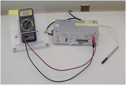
Figure 6: Close up of the Hall probe and readout. (The Hall probe is the pencil-like device to the right.)
6
The total shift will be a few millivolts. (Note that this is about ~1 Gauss, the size of the Earth's field.)
If the fluctuations in your probe are more than about 10 millivolts, you may have trouble with this part.
Make certain the filter is on and the connections are solid.
7
Record the conversion factor for your probe (1 volt reading with x100 setting on box = 100 Gauss). Leave the multimeter connected for later sections. How might you change the apparatus to make the Hall probe more sensitive? Think about the factors that affect the voltage reading in a Hall measurement; would more carriers (larger n) increase the Hall voltage? Larger current? A thicker/thinner Hall bar?
Field of a Circular Coil
1
Position the coil on the tabletop so that its axis is perpendicular to the Earth's field. One of the lab partners may have to hold the coil steady during these measurements.
2
Connect the DC Power Supply to the coil with test leads. Set the current to 1.0 amp. Investigate first the field direction, using the magnaprobe (or compass). Verify that the field lines encircle the wires of the coil, by watching the field direction as you loop the probe through the center and around the coil. Make a rough sketch of the field line distribution on the field-line mapping template. This need not be as exact as the permanent magnet map, but indicate on your sketch the direction of circulation of the current, and the direction of the magnetic field.
3
Align a meterstick with the coil axis and place the meterstick zero at the coil center. The coil should be on its side on the lab table. Use the Hall probe to measure the field along this axis. For this, leave the Hall probe range on xl00, and the multimeter on 200 mV. Readings should be taken with the probe tip facing the coil to obtain the maximum reading. (You have oriented the coil so that the Earth field contribution will almost vanish.) Record eight values of field and position, moving the Hall probe along the coil axis, starting at the coil center and ending about 20 cm from the coil. The field should decrease to about zero for the furthest reading. If not, the zero of the Hall probe might need to be readjusted. Enter these eight measurements into a table in an Excel spreadsheet.
4
Using the graphing feature of Excel, make a plot of the circular-coil magnetic field you have measured vs. position, on a linear scale. Plot the field in units of Tesla, converted from the voltage units of your measurements.
5
The large circular coil contains 200 turns, extending from a radius of 5.15 cm to 5.55 cm; take the average radius to be 5.35 cm. The winding extends 1.6 cm along the axis, but the geometry is very close to that of an ideal circular coil. Knowing the current and geometry, calculate the magnetic field expected at the center of the coil (Equation 3B =
.
). Place this theoretical point on the graph you have just made.
| μ0NIR2 |
| 2(x2 + R2)3/2 |
6
Based on the general formula for the field from a circular coil, (Equation 3) if we take the log of both sides of this equation and then plot the ln(B)
versus ln(z2 + R2),
we should get a straight line. Using your data in Excel, calculate these values for your coil and make the scatter plot and then add the linear trend line. From the linear fit, find the slope of the curve and its intercept.
7
How does your fit compare to the theoretical curve? Discuss your results.
Magnetic Fields and Materials
Magnetic field lines penetrate some (not all) materials.
1
Use the setup from steps 1-6 in Field of Circular Coil. Make sure that the probe tip faces the center of the coil, with about 5 cm spacing between the coil and the probe so that materials can be inserted in the gap.
Note: The aluminum block is made of a structural alloy, and is a good conductor (although roughly twice the resistivity of pure aluminum). The steel sheet has a thin coating of zinc (galvanized for rust resistance), but it consists mostly of steel (an iron alloy). The plastic block is a very good electrical insulator.
2
Turn the power supply current to 1.0 amp. Measure the magnetic field approximately 1.0 cm above the top of the coil when the following are placed between the top of the coil and the Hall probe:
-
awhen the insulating plastic block is placed on the top of the coil
-
bwhen the aluminum block is placed on the top of the coil
-
cwhen the steel sheet is placed on top of the coil
You will need to hold each material in place for a few seconds to reduce the random fluctuations in the reading.
Lastly, take the small iron "keeper" for the permanent magnet and place it inside the coil under the location of the Hall probe with its long dimension in the direction of the magnetic field of the coil and measure the field in the same location as your other measurements. Record these magnetic field measurements in a table.
Write a short explanation of these 4 measurements and what they imply about the magnetic properties of these materials.
3
Note that the behavior you observe characterizes the steel sheet as paramagnetic. Paramagnetic material can be identified by the attraction to either pole of a magnet (whereas another magnet will be attracted or repelled depending on the pole orientation). In paramagnetic materials, B fields induce internal currents having the direction that produces attraction. Induced fields tend to concentrate magnetic field lines, since they always present the "opposite" pole in response to the applied field resulting in magnetic attraction between the objects. Figure 7 illustrates these two behaviors, showing how these magnetic materials can be used to shield a region from magnetic field or to concentrate the field in a particular region.
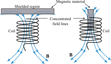
Figure 7
Strength of Permanent Magnets
1
Use the Hall probe, but change the sensitivity switch to x10, since these magnets are strong enough to saturate the probe on the more sensitive scale. Remove the keeper bar from the horseshoe magnet, and find the field at one pole. Repeat for the cylindrical magnet.
2
Record the maximum reading (in volts) for these magnets, and convert to a field strength in T.
3
Note that both magnets are made of alnico (alloys of iron, aluminum, nickel, and cobalt); do they have about the same strength? Make a table of the field strengths for these materials, ordering them from highest to lowest field values.