Vector Addition

Introduction

All measurable quantities may be classified either as vector quantities or as scalar quantities. Scalar quantities are described completely by a single number (with appropriate units) representing the magnitude of the quantity; examples are mass, time, temperature, energy, and volume. For vector quantities, such as velocity, force, and acceleration, the magnitude is accompanied by a directional quality. (Vectors will be denoted by A and unit vectors by î.) When scalar quantities are used in calculations, the ordinary rules of arithmetic apply; but when vector quantities are involved, the process is more complex since the direction of the vector must be taken into account. In this experiment, three methods for vector addition, graphical, analytical, and experimental, will be examined.

Theory

A vector quantity can be represented graphically by a straight line with an arrowhead at its end. The direction in which the arrow points gives the sense of the vector and the length of the line indicates the vector's magnitude. For example, a force of 3 N acting horizontally might be described by a line three units long (each unit representing 1 N) as shown in Figure 1.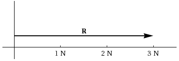

An arrow, which is labeled R, points to the right.

Figure 1: Vector R has both magnitude and direction.

When two or more vectors are used to describe a process, they can be replaced by a single resultant vector that carries the equivalent information. As an example, consider a car which travels from point O to point P, first by moving 50 km northwest, then 20 km west, and finally 40 km north. Now, instead of moving to point P in a series of three steps, represented by the vectors A, B, and C, the car could follow the more direct path shown by the vector R. This vector R, called the resultant, is equivalent to the combination of the three vectors A, B, and C since the car still begins at point O and ends at point P. This can be written symbolically as

( 1 )

R = A + B + C.

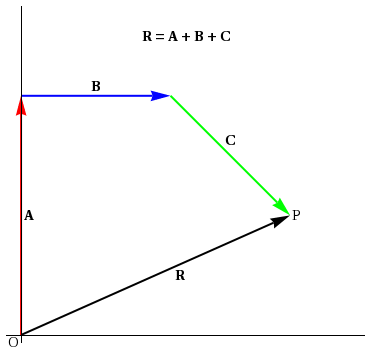
Figure 2: Graphical addition of vectors A, B and C

It should be noted that in this case all paths that represent movement from O to P are equivalent to R and to each other. So in Figure 3,

( 2 )

R = A + B + C = C + A + B = C + D.

Graphical addition of the vectors A, B and C from figure 2 showing C + A + B and A + B + C and C + D, where D is the resultant of A + B. All three of these yield the same resultant R.

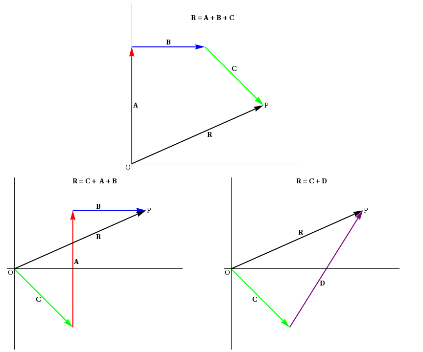
Figure 3: The same resultant R is obtained regardless of the order in which the vectors are added.

Although this graphical method, in which successive vectors are placed head-to-tail, is useful as a visual description, it is limited in precision by that which can be obtained by the drawing instruments. When results more accurate than those provided by graphical analyses are required, analytical methods are applied. In order to use analytical methods for vector addition, all vectors are described through the use of unit vectors. A unit vector is a vector having a magnitude of one (unaccompanied by any units) with a set orientation. Its only use is as a description of a specific direction in space. In the x-y coordinate system, it is the usual practice to assign the unit vector î in the direction of the positive x-axis and the unit vector ĵ in the direction of the positive y-axis. Any single vector can be expressed as the sum of two (or more) component vectors. In Figure 4, the vector A has a magnitude of A and an orientation of θ from the x-axis.

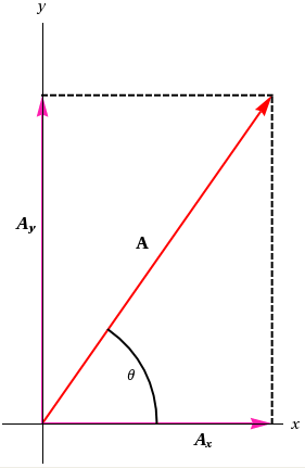
Figure 4: Vector A graphically resolved into components A_x and A_y.

This vector can be considered to be the resultant of two component vectors: A_x = A_xî pointing along the î direction and A_y = A_yĵ pointing along the ĵ direction; or symbolically as follows.

( 3 )

A = A_xî + A_yĵ

( 4 )

A = A_x + A_y

The component A_x is positive or negative as A_x is in the +î or –î direction, and A_y is positive or negative as A_y is in the +ĵ or –ĵ direction. The magnitude of the components of A can be calculated from the definitions of trigonometric functions

( 5 )

sin θ =

A_y

( 6 )

A_y = A sin θ

and

( 7 )

cos θ =

A_x

( 8 )

A_x = A cos θ.

In addition,

( 9 )

tan θ =

A_y

A_x

( 10 )

θ = arctan

A_y

A_x

and by the Pythagorean theorem, the magnitude of A is

( 11 )

|A| =

A_x² + A_y²

When vectors are added analytically each vector is first written in its component form, then the x-components of all the vectors are added algebraically (paying strict attention to sign) to obtain a resultant x-component, and the y-components of all the vectors are added to give the resultant y-component. Suppose two concurrent vectors are added. For the head-to-tail graphical method, the vector B is placed at the arrowhead of the vector A (or vice versa) and the resultant, R, is drawn from O to the tip of B as shown in Figure 5.

The first of two diagrams shows vectors A and B on a coordinate axis, with both having their tail at the origin. The second diagram shows B redrawn with its tail at the tip of the original vector A. Vector R is drawn from the tail of A to the tip of the redrawn B. To show that the order does not matter, vector A has also been redrawn with it's tail at the tip of the original vector B. So it looks like a parallelogram with the vector R along one of the diagonals.

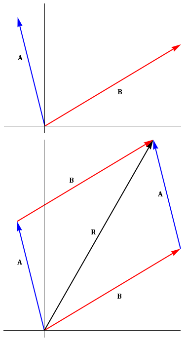
Figure 5: Graphical vector addition of two vectors

In Figure 6, the vectors C and D are added analytically. In mathematical terms, the vectors can be written

( 12 )

C = C_xî + C_yĵ

( 13 )

D = D_xî + D_yĵ

( 14 )

R = R_xî + R_yĵ.

Figure 6: Vectors C and D resolved into components graphically and analyically, along with their resultant vector R.

Since the resultant, R, is the sum of the vectors C and D

( 15 )

R = C + D

( 16 )

R = C_xî + C_yĵ + D_xî + D_yĵ

( 17 )

R = (C_x + D_x)î + (C_y + D_y)ĵ.

A comparison with equation (14) gives the values for the x-and y-components of the resultant:

( 18 )

R_x = C_x + D_x

( 19 )

R_y = C_y + D_y.

From the components of R, the magnitude and direction of the resultant are

( 20 )

|R| =

R_x² + R_y²

( 21 )

θ = arctan

R_y

R_x

If more than two vectors are being added, equations (18) and (19) can be generalized to

( 22 )

R_x = A_x + B_x + C_x + D_x +

( 23 )

R_y = A_y + B_y + C_y + D_y +

and the relationships of equations (20) and (21) can be applied to obtain the magnitude and direction of the resultant. When the vectors being added represent forces, the negative of the resultant is called the equilibrant (or antiresultant) of the forces. The equilibrant is the single force that, in combination with the other forces, will bring the system into equilibrium. Note that the equilibrant is equal in magnitude but opposite in direction to the resultant of the vectors.

Objective

The objective of this laboratory is to find the equilibrant force for one or more known forces using the force table, and to compare this result to those obtained using graphical and analytic methods.

Apparatus

Ruler protractor
Three pulleys
Slotted mass set
Three mass hangers
Force table with center pin and ring
Bubble level

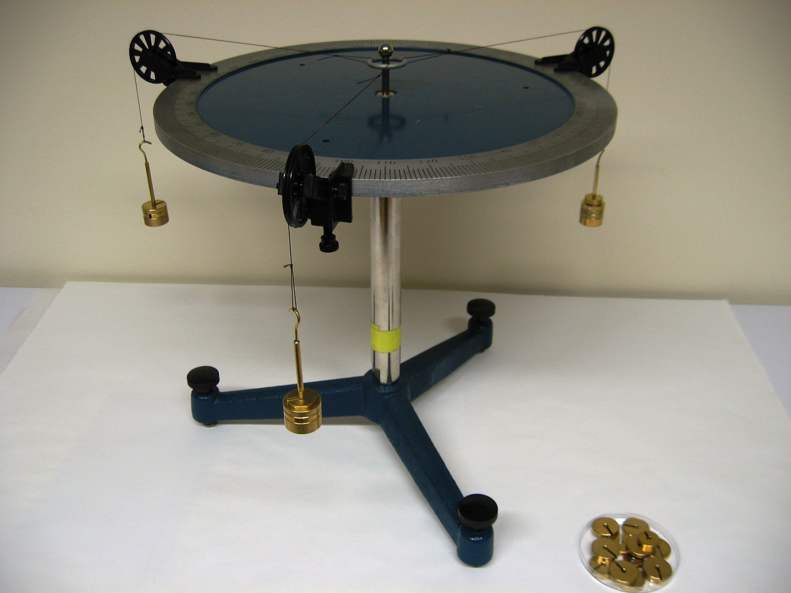
Figure 7: Apparatus

Procedure

Please print the worksheet for this lab. You will need this sheet to record your data.

The force table consists of a horizontally mounted surface that is graduated in degrees along its perimeter. A pin inserted at the center of the table holds a ring in place when the system is unbalanced. The ring is the object that will be placed in equilibrium and the tensions of the three strings attached to it will provide the forces to be balanced. Provided the friction in the pulleys is negligible, the tension in each string is equal to the downward weight of the mass placed at its ends (this will be a topic of further discussion in class). The pulleys may be clamped at any desired angle and the direction of each force is indicated by the position of the pulley index mark on the circular scale of the table.

A: Experimental Method for Determining the Resultant of Two Vectors

Before using the force table it is important that it be level. Use the bubble level to check that the force table platform is horizontal. If it is not, use the leveling screws to make necessary adjustments until the surface is horizontal.

Using the values provided by WebAssign for Case 1, arrange the pulleys at the angular positions of the two vectors given on the diagram.

Caution:
Please note that it is very easy to over tighten the clamps holding the pulleys to the table surface, so be careful to tighten these clamps only a fraction of a turn once the clamp contacts the table surface (finger tight).

Suspend the weights listed for each vector over the corresponding pulley. Be sure to include the weight of the holder when calculating the mass on the strings. Once these weights are in place, use the third pulley and weight system to find the equilibrant vector associated with the two vectors that you have been given. Adjust the angle of the force on the table as well as the mass until you have found the equilibrium configuration.

Gently tap the ring to displace it slightly from the center; if the ring returns to its original position then it is in equilibrium. When the ring appears to be in equilibrium, carefully remove the central pin and once again tap the ring to displace it slightly. If the ring does not return to the center position, replace the central pin and readjust the mass and position of the pulley for the equilibrant until equilibrium is established. For a body in equilibrium, the net force acting on the body is zero. For the three vectors represented on the force table

A + B + C = 0

A + B = −C,

where C is the equilibrant. The resultant, R, of the two vectors on the assignment card is

R = A + B

R = −C

and the resultant is the negative of the equilibrant.

Record the position of the equilibrant to a fraction of a degree and record its magnitude to the smallest mass available. Sketch the vector arrangement as it is drawn on the assignment card and include the equilibrant found from the force table on the diagram. Keep the angle of the equilibrant fixed.

Keep the angle of the equilibrant fixed. In order to find the experimental uncertainty for the magnitude of the equilibrant, add to (or remove from) the pulley enough weight to cause the ring on the force table to depart significantly from its equilibrium position. The amount by which the mass was changed is a measure of the experimental uncertainty in the vector magnitude. Record this uncertainty to the smallest mass available (be sure to include the proper units).

Place the ring in equilibrium once again. Keeping the magnitude of the equilibrant fixed, find the experimental uncertainty in the direction of the equilibrant by moving the pulley slightly until the ring is no longer in equilibrium. The change in the angle necessary to remove the ring from its equilibrium position represents the experimental uncertainty in the direction of the equilibrant. Record this uncertainty to a fraction of a degree.

Repeat procedures 1–5 for Case 2.

B: Graphical Method for Determining the Resultant of Two Vectors

On a sheet of linear graph paper, add the two vectors shown in the case using the head-to-tail method described in Figure 3.

Draw the vectors to scale (using as large a scale as possible) and accurately measure off the angle with the protractor provided.

Draw the resultant and equilibrant on the diagram and measure and record the magnitude and direction of the two vectors. Do this for both cases.

C: Analytical Method of Determining the Resultant of Two Vectors

On a set of x-y coordinate axes, draw approximately to scale and in any convenient orientation the two vectors listed in the case. Resolve each vector into its x- and y-components and list them in the table above the sketch.

From these values, obtain the x- and y-components for the resultant and, using equations (20) and (21), determine the magnitude and direction of the resultant and draw it on the sketch. Do this for both cases.

D: Calculations

Determine the % error for the magnitude of the resultant obtained by the experimental and analytical methods.

Determine the % difference for the magnitude of the resultant obtained by the experimental and graphical methods.

E: Questions

Concurrent forces are forces that act at a single point. The assignment cards show concurrent forces but the forces on the force table act on a ring, not at a point. Nonetheless, the forces are still concurrent. Explain.

Could all three pulleys on the force table be placed in one quadrant and still be in equilibrium? Explain.

Suppose three forces with magnitudes of 220 N, 270 N, and 200 N are placed in equilibrium. If the 200 N force acts in the +y-direction, what are the two configurations in the xy-plane that the remaining forces may have? Give numerical values for the angles and show your results on a sketch.

What is the condition necessary for equilibrium (consider only linear motion)?