Vibrating Strings

Introduction

Stationary waves are the underlying basis for most musical instruments, for example: guitar, violin, flute, etc. The quantized nature of standing wave generation results in a direct correspondence between integers and musical notes, a fact known to the ancient Greeks, in particular Pythagoras, who claimed that their beauty was a result of this fact.

An interesting phenomenon occurs when a wave is set up on a string with both ends fixed and not allowed to oscillate. If the length of the string coincides exactly with

, ...,

of a wavelength of the wave then a stationary wave pattern will be set up in the string (Figure 1(a)). If the length of the string does not permit

wavelengths along the length of the string, then the waves traveling in either direction after reflection from an end will be out of phase and destructive interference will be observed, resulting in no pattern (a relatively smooth and straight string) (Figure 1(b)).

2 figures labeled (a) and (b) each with 3 images. The first image in (a) has a dashed horizontal line extending to the left from the midpoint of a vertical bar. 2 sine curves symmetric with each other about the dashed line originate from the bar, intersect each other at the dashed line twice, and end at a third intersection forming 3 regions. Beneath the first region a horizontal arrow points away from the bar. Above the last region a horizontal arrow points toward the bar. In the second image the 3 regions are solid with dashed boundaries. The third image is a horizontal double arrow bounded at end by a vertical line spanning the length of the three regions. Text above the arrow reads L = 3 lambda / 2. The first image in (b) is like the first image in (a) except the curves are asymmetric and do not intersect each other at the dashed line. The second image is of a single slightly curving line extending from a horizontal bar. The third image is like the third image in (a) except the text reads L not equal to n lambda / 2.

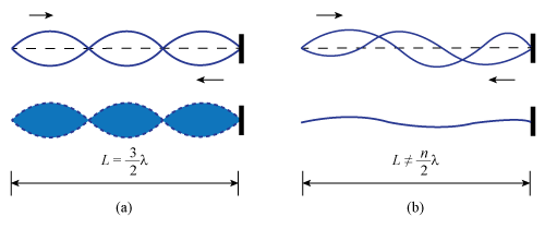
Figure 1

In Figure 1(a), the points of maximum amplitude are called antinodes and the points in the pattern that remain motionless are called nodes. The distance between antinodes is

where λ is the wavelength. Therefore, the condition for a standing wave on a string fixed at both ends is

( 1 )

L =

where n is the number of segments (also the number of antinodes) in the pattern. The velocity, v, of a transverse wave on a string is given by

( 2 )

v =

where T is the tension in the string and μ is the linear mass density (mass per unit length) of the string. In our experiment, the tension in the string will be provided by the weight of the mass, M, suspended at the end of the string. Therefore,

( 3 )

v =

For any type of wave the relationship between the velocity, v, of the wave, its frequency, f, and its wavelength, λ, is given by

( 4 )

v = fλ.

Combining Equations (1), (3) and (4), we obtain the following expression governing stationary waves on a string.

fλ

( 5 )

4f²L²

n²

Rearranging gives

( 6 )

L²

4f²

n²

In this equation n is the number of segments (antinodes) in the stationary pattern and L is the total length of these n segments. In this experiment we will set up several standing (stationary) wave patterns. By varying n (by adjusting M) and μ (by using strings of varying thickness) and measuring L in each case, we can plot an appropriate graph and use its slope to calculate the frequency, f, of the wave. We will compare this calculated value to the actual frequency of the wave as generated by the motor used to create the waves.

Objective

In this experiment we will make measurements for standing wave patterns on a string. Graphical analysis of our data will allow us to calculate the frequency of the waves on the string. We will compare our calculated frequency to the known frequency and in this way we will test the validity of the three equations presented in the lab manual:

v = fλ, v =

, and L =

λ.

Apparatus

String vibrator (motor) with two strings attached
Mass hanger
Slotted mass set (plus 1, 2, and 5 gram masses on top of outline sheet taped to lab table)
Meterstick
Strobe light (one per room)

Procedure

Please print the worksheet for this lab. You will need this sheet to record your data.

Take the black string, pass it over the groove in the pulley and hang the mass hanger from the end of the string to temporarily hold the string in place. Plug in the motor (vibrator). Recall that according to Equation (5), increasing the number of nodes, n, requires a decrease in the mass, M, attached at the end of the string. The mass of the hanger is 50 grams. The mass, M, is the total mass suspended from the string, the mass of the hanger plus the mass of the slotted masses placed on the hanger.

Two things to keep in mind are:

i
Since one end of the string is attached to the motor, the segment (oval-shaped part of the string that consists of a node-antinode-node) connected to the motor must be neglected, because the motion at the motor prevents a true node from forming at that end. Therefore, whenever n segments are counted the last one, the one next to the motor (vibrator), is neglected. When the length, L, of the standing wave pattern is measured, the neglected segment adjacent to the motor is not included. See Figure 2.
ii
Standing waves are a quantized phenomenon. The standing wave pattern appears only at precise values of M and disappears if M deviates by just a few grams. So, M must be adjusted with precision. A good trick for finding standing wave patterns is to pinch the string (using your fingers) just above the attached mass (below the pulley). Use your fingers to increase or decrease the tension by small amounts to search for a particular pattern and then adjust M accordingly.

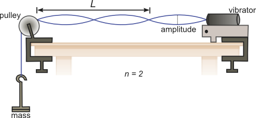
A table is set up with the experimental apparatus including a string vibrator, and a string hanging over a pulley with a mass at the end. The string is in a standing wave pattern with small amplitude. The string has n = 2 nodes since the end of the string attached to the vibrator doesn't count as a node due to the motion of the motor. The length, L, of the string is determined by the distance from the first node of the string to the last node located at the pulley.

Figure 2

Start with the black string and search for the

n = 1

pattern. Adjust the mass on the hanger in small increments until the required standing wave pattern is found (remember that the segment next to the motor is neglected). Keep adjusting the mass until the maximum possible amplitude (widest vertical separation for the antinode) is achieved. Measure and record in Table 1 in your worksheet the mass, M, that generates the

n = 1

pattern. Note that M is the total mass suspended from the end of the string, the mass of the hanger plus the total mass of the slotted masses on the hanger. Measure the total length, L, of the pattern with n segments (omitting the one next to the motor) and record this value of L in the table.

Repeat this procedure for both strings and for all values of n that are listed in Table 1. The black string has mass per unit length 0.0014 g/cm and the white string has mass per unit length 0.0033 g/cm.

Fill in the

n²

and

L²

columns of the table. Recall that Excel is available on the computer to assist with doing the calculations. Use Excel to plot a graph of

L²

vs.

n²

using the values you entered in Table 1. Your plotted points should fall close to a straight line that passes through the origin. If they do not and you and your lab partner can't find what is wrong, ask the TA for help.

Use Excel to find the slope of the straight line that gives the best fit to your data. Enter the results in your worksheet.

Assume

g = 980 cm/s².

Use the slope from your graph to calculate the frequency, f.

The actual value of the frequency is

f = 120 Hz.

This value can be determined using a stroboscope, which your TA will demonstrate at the end of the lab. Calculate the percentage error in your experimental measurement of f,

( 7 )

percentage error =

|actual - experimental|

actual

× 100%,

where the experimental value is the one calculated using the slope of your graph.