Statistical Analysis of Data Collected

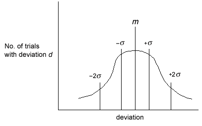
When performing laboratory experiments, a certain variation in results will always occur regardless of the care taken in measuring. Though all systematic errors have been avoided, the student will notice that the values obtained will deviate from each other. Random errors are unavoidable. Variations occur because each measurement is subject to the sensitivity of the measuring instrument and/or the estimation of the experimenter. Examples: Sample masses determined using an analytical balance to determine the sample mass has a precision of ±0.0001 g. Each of the two buret readings used to determine the volume of titrant has a precision of ±0.02 mL. Finally, the experimenter's estimation of the endpoint is ±0.03 mL minimum. These sources of error can either add or cancel each other, producing the normal distribution (bell) curve shown. The individual trials vary about the average (mean). The challenge is to determine which trials to use and which should be discarded.

Test for Discarding Outlying Results

4D Test

Average all trials EXCEPT the outlying value.

Determine the average deviation of the trials retained.

If the deviation of the outlying value is greater than four times the average deviation, the sample potentially can be discarded.

Perform several additional trials. With a larger sample size, one can feel more confident in discarding data if all results except the outlier are in close agreement.

Standard Deviation

The standard deviation for a small set of data will generally be larger than the average deviation since only a small part of the normal distribution curve has been sampled. The two deviations will approach each other as the number of trials increases. The STANDARD DEVIATION is generally better to use since this small sample size is taken into account by dividing by n – 1 rather than n trials.

Normal Distribution Curve

One standard deviation (±1σ) contains 68.3% of data. Two standard deviations (±2σ) contain 95% of data. Three standard deviations (±3σ) contain 99.7% of data. Four standard deviations (±4σ) contain 99.9+% of data.

Figure

Sample Calculation

Sample Data

Statistical Analysis of Data

4D Test

Compute average "good" values (all except outlier).

0.3221 + 0.3231 + 0.3218
3
= 0.3223 M

Compute the average deviation of "good" values. (Note: deviation is the absolute value of the difference from the mean.)

|0.3221 − 0.3223| = 0.0002
|0.3231 − 0.3223| = 0.0008
|0.3218 − 0.3223| = 0.0005
0.0015/3 = 0.0005

Compute the deviation of outlying value, and compare it to 4D or 4 × average deviation.

|0.3561 − 0.3223| = 0.0338 compared to: (0.0005) = 0.0020
0.00338 > 0.0020

∴

Based upon the 4D test, results MAY be discarded.

Once results that may be discarded have been determined, the standard deviation can be calculated.

Standard Deviation

( 1 )

s =

	(x₁ − m)²

n − 1

	x_i = sample value
	m = mean
	n = number of trials

m =
0.3221 + 0.3231 + 0.3218
3
= 0.3223 M
s =
((0.3221 − 0.3223)² + (0.3231 − 0.3223)² + (0.3218 − 0.3223)²
3 − 1
s =
(4E⁻⁸ + 6.4E⁻⁷ + 2.5E⁻⁷⁾
2
= 6.8E⁻⁴ (calculator)

Final answer: 0.3223 ± 0.0007 M. (In your final answer, express your standard deviation to one significant figure and your molarity to four significant figures.) You can also calculate standard deviation using your calculator:

•
You will need to put lists of information (DATA) into your calculator. Do this by pressing STAT 1:Edit.
•
Enter your data in one of the columns, for example, L1.
•
Now go to STAT > CALC and select 1:1-Var Stats.
•
Enter L1 (2^nd 1).
•
Sx is the standard deviation, which for this example is
6.806859E⁻⁴
(express as 0.0007).

You will also calculate % error and % accuracy in many of the labs

The % error is how "far off" your results are.

( 2 )

% =

theoretical − experimental

theoretical

x 100

The % accuracy is how "close" your results are.

( 3 )

% =

experimental

theoretical

x 100

\|0.3221 − 0.3223\|	=	0.0002
\|0.3231 − 0.3223\|	=	0.0008
\|0.3218 − 0.3223\|	=	0.0005
		0.0015/3 = 0.0005