The RC Circuit

Introduction

The goal in this lab is to observe the time-varying voltages in several simple circuits involving a capacitor and resistor. In the first part, you will use very simple tools to measure the voltage as a function of time: a multimeter and a stopwatch. Your lab write-up will deal primarily with data taken in this part. In the second part of the lab, you will use an oscilloscope, a much more sophisticated and powerful laboratory instrument, to observe time behavior of an RC circuit on a much faster timescale. Your observations in this part will be mostly qualitative, although you will be asked to make several rough measurements using the oscilloscope.

Part 1: Capacitor Discharging Through a Resistor

You will measure the voltage across a capacitor as a function of time as the capacitor discharges through a resistor. The simple circuit you will use is shown in Figure 1. The capacitor, C, is an electrolytic capacitor of approximately 1000 µF or 10^–3 F, with a manufacturing tolerance of ±20%. The resistance of the resistor, R, is 100 kΩ (10⁵ ohms), with a tolerance of ±5%. DMM represents the digital multimeter used to measure DC voltage across the capacitor. The idea is simple: by closing switch S, you will charge up the capacitor to approximately 10 volts using the adjustable power supply. The capacitor is connected in parallel with a resistor, so that when you open the switch the capacitor will begin discharging through the resistor. Using a stopwatch and multimeter, you will record the capacitor voltage every 20 seconds until the capacitor has almost completely discharged. The goal is to examine the exponential decay of this RC circuit.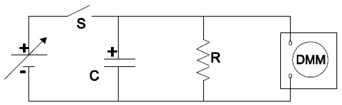

Figure 1

Part 2: The Series RC Circuit and the Oscilloscope

We shall use the oscilloscope to study charging and discharging of a capacitor in a simple RC circuit similar to the one shown in Fig. 2. In place of the multimeter used in the first part of lab, the oscilloscope will be used to measure the voltage across the capacitor. More about the oscilloscope can be found in Reference: The Oscilloscope.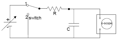

Figure 2

Assume the capacitor has zero charge on its plates and the switch is then put in position 1 as shown. This puts the resistor and capacitor in series with the power supply. Current flows and the capacitor charges up. How does the magnitude of the resistance affect the speed of charging? If R is small, then when the switch is initially switched to position 1, current will flow easily and the charge Q on the capacitor will build up quickly. Simultaneously, the potential difference across the capacitor increases until it equals the potential difference applied to the circuit from the power supply, V_emf. Current will then no longer flow. If on the other hand, R is large, then a smaller current flows initially and it takes a longer time for the capacitor to charge.

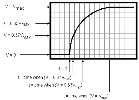
Figure 3: A Charging Capacitor

It can be shown theoretically that the voltage across the charging capacitor in the circuit described above is the following.

( 1 )

V_C = V_emf(1 – e^{–t /RC})

This discussion is correct only for the charging of the capacitor. What happens if the switch is now moved to position 2? This takes the power supply out of the circuit. The capacitor now discharges through the resistor until there is no potential difference between the plates. This is the same situation you studied in Part 1. The voltage across the discharging capacitor is given by the following.

( 2 )

V_C = V_emfe^{–t /RC}

The product RC is called the time constant. With the switch in position 2, V_R = V_C. Later, at t = RC, the voltage across the resistor V_R = V_emfe^–1 = 0.3679V_emf. After this time, the potential difference across the resistor has been reduced to about 37% of its initial value, V_emf. You will observe the potential difference across the capacitor as a function of time for a circuit containing a charging and discharging capacitor. Using this data and equation above, you can estimate the value of the product RC and compare this value with the known value of RC.

Why find the time constant? The time constant is a characteristic of all exponential curves and tells us, in a single number, how fast or slow the curve is rising or decaying. For any exponential function, knowing the time constant tells us how long it takes for that function to fall to 1/e, or ~37%, of its initial value for a decay; or how long it will take for a rising exponential function to reach (1 – 1/e), or ~63% of its final value. For example, under ideal conditions, the number of bacteria in a culture grows exponentially, and the growth can be described by an exponential equation: N(t) = N₀e^kt, where N₀ is the number of bacteria initially present, N(t) is the number present some time t later, and k is the time constant, indicating how fast the culture will grow.

Procedure

Part 1: Capacitor Discharging Through a Resistor

1
Fully discharge your capacitor. Measure the capacitance of your capacitor using the capacitance meter provided by your instructor. Note the accuracy rating for the capacitance meter you used (see Appendix - Instrument Accuracy), and use this to estimate the uncertainty of your reading. Measure also the resistance of the resistor using the multimeter, and look up the accuracy of the meter for the range you used.
2
Again, make sure the capacitor is fully discharged. Assemble the circuit shown in Fig. 1 using banana plug cables. NOTE THE CAPACITOR HAS + AND – LEADS. Be sure the + end is connected to the positive (RED) connector on the power supply and the – end is connected to the negative (BLACK) connector.

Caution:
THE CAPACITOR WILL EXPLODE IF LEFT CONNECTED BACKWARDS TO THE POWER SUPPLY.

3
Turn on the digital multimeter and set the selector switch to measure DC voltage. Locate the Data Hold button on the meter, labeled either DATA-H or DATA HOLD. When this button is pushed once, the meter display "freezes" to display the voltage present when the button was pushed. A DH symbol will appear in the display. Pushing the Data Hold button again releases the display to show the current circuit voltage.
4
Turn on the power supply with the control knob fully counterclockwise (zero). Close the switch. Turn the power supply control knob clockwise until the voltage across the capacitor and resistor is approximately 10 volts, as indicated on the multimeter.
5
When the control knob is set where you want it, measure the charged capacitor voltage. Record this value as your starting voltage, V₀, for time t = 0.
6
One lab partner should be ready to write down the voltages called out by the other partner, who will be watching a stopwatch and taking voltage readings. When you're ready to begin, simultaneously open the switch and begin timing.
7
At successive intervals of 20 seconds (20 s, 40 s, 60 s, etc.), push the Data Hold button to read the voltage. Record each voltage, V_C, and time, t. Push the button again to release the display and be ready for your next reading. Continue taking readings until at least five minutes (300 seconds) have elapsed.
8
Take two additional readings at one minute intervals, e.g. at 6 minutes and 7 minutes. By now the capacitor voltage should be nearly zero.

Part 2: The Series RC Circuit and the Oscilloscope

In this experiment, a function (or signal) generator shown in Figure 4 will replace the switch and power supply shown in Figure 2. This is only a minor difference, and one that you don't need to worry too much about. In essence, the function generator has the effect of "opening and closing the switch" many times every second in a regular and repeatable way. This allows us to use an oscilloscope to measure the time dependence of the voltage.

1
Measure and record the resistance (R = 5.6 kΩ, nominal value) of the resistor with the multimeter and the capacitance (C = 1 nF, nominal value) of the capacitor with the capacitance meter provided. The accuracy of the capacitance meter is listed in the Appendix.
2
Connect the function generator, capacitor, resistor, and oscilloscope O as shown in Figure 4. Connect the leads from the oscilloscope so that they are measuring the potential difference across the capacitor. Note connections for the positive and negative leads.

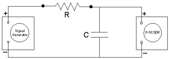
Figure 4

3
Set all the controls on the scope as instructed in the oscilloscope exercises in Reference: The Oscilloscope. Set the sweep rate to 50 µs/div. Set the frequency on the signal generator to about 8 kHz and make sure it is set to produce square waves.
4
Turn on the scope and the function generator. Increase the amplitude on the function generator to about half of the maximum. Adjust the gain (volts/div) and the sweep (time/div) knobs on the scope until you see a trace that looks something like Fig. 3. It may be necessary to fine-tune the "trigger level" setting to get a clear display. Be sure that you can see the point corresponding to t = 0. Adjust the vertical shift knob on the scope and the amplitude knob on the function generator until the maximum and minimum voltage levels of the trace are aligned with the top and bottom horizontal grid lines (graticules) on the screen. Shift the horizontal position of the trace until the beginning of the charging or discharging curve lines up with a vertical graticule. This alignment with the grid lines makes it much easier to read measurements from the scope. Have your instructor check your display before you go further.
5
Using the beginning of the decay as the t = 0 point, measure the amount of time it takes for the capacitor voltage to decay to 37% (e^–1) of its maximum value at t = 0. Alternatively, you could measure the time it takes for the capacitor to charge to 63% of its maximum value. Either measurement gives the RC time constant for the circuit. If your scope's sweep function has a magnification switch (10x), you may be able to obtain a more precise measurement by expanding part of the trace to fill more of the screen.
6
Temporarily turn off the function generator and remove the 5600-ohm resistor from your circuit. Replace it with a resistor substitution box set to approximately 5600 ohms. Turn the function generator back on and again observe the trace on the oscilloscope. Now change the resistance value and observe how the charging/discharging curve changes. Qualitatively note what happens when you make R much larger or smaller than the original value of 5600 ohms.

Be sure that you and your T.A. initial your data sheet.

Analysis

1
Make a plot of ln(V_C/V₀) vs. t from the data obtained in Part 1. Enter your time data in units of seconds.
2
The equation for the capacitor voltage as a function of time is given as
V_C = V₀e^−t/RC.
Make a least-squares linear fit of your plot of ln(V_C/V₀) vs. t. Identify the parameters used in the fit to the equation for the exponential decay of the capacitor voltage.

Discussion

For both parts of the experiment, compare the value of the time constant obtained to the predicted value, computed from the known values of R and C. Is the agreement to within the accuracy of the value for RC measured using the capacitance and multimeter?