
Measuring the Rydberg Constant
Introduction
In this experiment, you will observe the visible wavelengths of light produced by an electric discharge in helium gas, using a diffraction grating. From knowledge of the wavelength values, you will be able to accurately calibrate the diffraction grating line spacing. Once calibrated, the grating is used to measure the wavelength of light produced by atomic hydrogen. By performing a curve fit to these measured wavelengths, you can determine the Rydberg constant, an important physical constant. This is an experiment in which careful technique and measurement will pay off: you should be able to determine the Rydberg constant to within one percent or better. The helium and hydrogen gasses are contained in low-pressure discharge tubes that have metal electrodes at each end. When a high voltage is applied across the two electrodes, an electric current flows through the gas. High-energy electrons in the electric current collide with gas atoms and, in the process, can impart internal energy to the atoms. These excited atoms can then release energy in the form of electromagnetic radiation at specific wavelengths. Some of this electromagnetic radiation is in the visible range. A Swiss schoolteacher named Johann Balmer (1825 - 1898) studied the wavelengths of visible light emitted by hydrogen atoms. He found an empirical equation that accurately matches the values of the observed wavelengths.( 1 )
| 1 |
| λ |
 |
| 1 |
| 22 |
| 1 |
| n2 |
 |

( 2 )
mλ = d sin θ
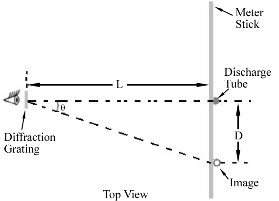
Figure 1
mλ = d sin θ
. Hence, different wavelengths will appear at different locations along the meter stick. The angle corresponding to each wavelength can be determined by measuring D and L.
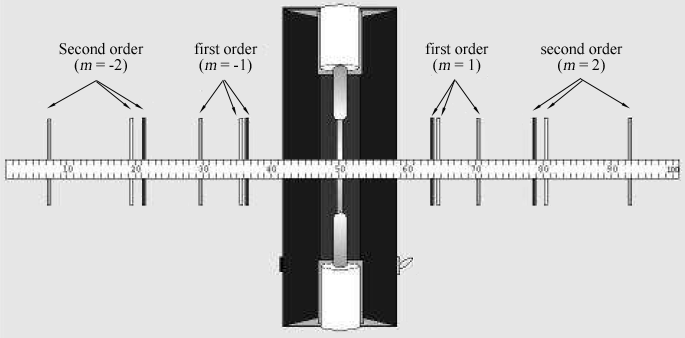
Figure 2: Spectral lines seen through the diffraction grating one meter from a discharge tube.
mλ = d sin θ
, then d can be determined. You will measure θ for seven known wavelengths in helium. A curve fit will then enable you to accurately determine the grating spacing d. In the second part of the lab, you will use this value of d to accurately measure wavelengths in hydrogen.
Procedure
Caution:
Use extreme caution around the discharge tube power supply. It produces 5000 volts with sufficient current to be dangerous. Do not touch the supply electrodes or the tube while the supply is turned on. Turn off the power supply when changing discharge tubes. Since the area gets very hot during use, avoid grabbing the middle of the tubes.
Use extreme caution around the discharge tube power supply. It produces 5000 volts with sufficient current to be dangerous. Do not touch the supply electrodes or the tube while the supply is turned on. Turn off the power supply when changing discharge tubes. Since the area gets very hot during use, avoid grabbing the middle of the tubes.
Part 1: Helium Spectrum
1
Set up the arrangement shown in Figure 1. Make sure the discharge tube power supply is unplugged and turned OFF. Insert a helium gas tube in the electrode holders. (The tubes are fragile; please handle them with care.) The tube should be straight up and down and positioned near the 50 cm mark on the meter stick.
2
Plug in and turn on the power supply. The discharge tube should immediately light. If it does not, ask you instructor for assistance. One lab partner should look through the diffraction grating while the other partner works on the opposite side of the meter stick taking readings.
3
The person looking through the diffraction grating should look left and right of the discharge tube to locate the diffraction images. Locate the first order (m = ± 1)
and second order (m = ± 2)
images. If necessary, rotate the grating so that the images appear just above and below the meter stick in the same way the discharge tube itself does.
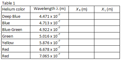
4
Table 1 lists the wavelengths of seven of the brightest visible lines in the helium spectrum in the order of shortest to longest wavelength. The images for each diffraction order will appear in this same order, with the smallest wavelength at the smallest angle. Match up the images with the wavelengths listed. Looking through the grating to the right, locate the position of the first image along the meter stick. The lab partner looking through the grating should instruct the other lab partner to position a small pointer (e.g., a pencil) along the meter stick
until the pointer is in line with the image being measured. The partner with the pointer then reads the position along the meter stick. Use a low-wattage reading lamp if necessary to read the meter stick. Record the position XR of each of the helium lines in Table 1.
5
Repeat the process for the seven images appearing to the left of the discharge tube. Record the position XL of each image in Table 1.
Part 2: Hydrogen Spectrum
1
Turn off and unplug the discharge power supply and allow the discharge tube to cool for several minutes. (Caution: The tube will be very hot when you first turn the supply off.) Remove the helium tube and replace it with the hydrogen tube. Position the power supply again with the hydrogen tube at the 50 cm position along the meter stick.
2
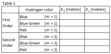
Three easily observed colors in hydrogen are listed in Table 2. Match the colors with the images seen through the diffraction grating. Record the positions XR and XL of the first order images in Table 2.
3
Without disturbing the meter stick or diffraction grating, carefully measure the distance L in Figure 1 using a metric tape measure. Include the uncertainty in your recorded value.
Analysis
Grating Spacing d
1
For each helium wavelength, calculate the average distance between the discharge tube and the first order images using the following equation.
( 3 )
D =
| XR − XL |
| 2 |
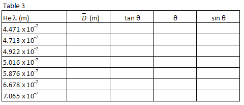
2
Also calculate tan θ =
, θ,
and sin θ for each wavelength. Record your calculations in Table 3.
| D |
| L |
3
Plot λ vs. sin θ and, using a least squared linear fit, find the slope. From the slope of your graph, find your best estimate for the grating spacing, d, in meters and the estimated error in d.
Rydberg Constant
1
Following the same procedure used in step 1 above, find sin θ for each of the hydrogen wavelengths you observed and record them in Table 4.
2
Using the value for the grating spacing found in step 2 above and the grating equation, Eq. (2)mλ = d sin θ
, calculate the wavelength, in meters, of the three hydrogen lines you observed and record
those in Table 4.
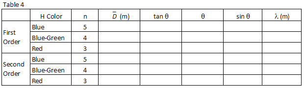
3
Table 4 lists the integer or "principal quantum number," n, associated with each of the
wavelengths you observed in hydrogen and which appears in the Balmer Equation (Eq. (1)| 1 |
| λ |
|
| 1 |
| 22 |
| 1 |
| n2 |
|
4
Perform a least square linear fit to your data.
5
Eq. (1)| 1 |
| λ |
|
| 1 |
| 22 |
| 1 |
| n2 |
|
( 4 )
| 1 |
| λ |
|
| 1 |
| no2 |
| 1 |
| n2 |
|
6
Compare this form to your curve fit equation to find values for the constants R and no. From
the error in the slope given by the curve fit, find the uncertainty for R.