Interpreting the Standard Deviation for Bell-Shaped Curves: The Empirical Rule

Once you know the mean and standard deviation for a bell-shaped curve, you can also determine the approximate proportion of the data that will fall into any specified interval. Here are some useful benchmarks.

68% of the values fall within 1 standard deviation of the mean in either direction.
95% of the values fall within 2 standard deviations of the mean in either direction.
99.7% of the values fall within 3 standard deviations of the mean in either direction.

Note: A small percentage, about 0.3%, falls farther than 3 standard deviations from the mean.

Combining the Empirical Rule with knowledge that bell-shaped variables are symmetric allows the "tail" ranges to be specified as well. The first statement of the Empirical Rule implies that about 32% of the values fall farther than 1 standard deviation from the mean in either direction. Due to the symmetry of the bell-shaped curve, we can say that about 16% of the values fall more than 1 standard deviation below the mean and about 16% fall more than 1 standard deviation above the mean. Similarly, about 2.5% fall more than 2 standard deviations below the mean and about 2.5% fall more than 2 standard deviations above the mean.

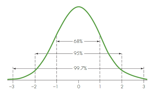
A graph with a bell-shaped, continuous, and symmetric curve above the horizontal axis is given.

There are 7 equally spaced labels on the axis; from left to right they are:
$-3$
,
$-2$
,
$-1$
,
$0$
,
$1$
,
$2$
, and
$3$
.

The curve enters the viewing window just above the axis at
$-3$
, reaches a peak at
$0$
, and exits the viewing window just above the axis at
$3$
.

A dashed vertical line is drawn above the numbers
$-3$
,
$-2$
,
$-1$
,
$1$
,
$2$
, and
$3$
.

"68%" is written on the line segment that extends from the dashed vertical line over
$-1$
to the dashed vertical line over
$1$
.

"95%" is written on The line segment that extends from the dashed vertical line over
$-2$
to the dashed vertical line over
$2$
.

"99.7%" is written on the line segment that extends from the dashed vertical line over
$-3$
to the dashed vertical line over
$3$
.

Identifying Possible Outliers

One guideline sometimes used to identify outliers is that data values more than 2 standard deviations in either direction from the mean are possible outliers. As an example, suppose that a sample of body temperatures (Fahrenheit) for people who are not ill has a mean of 98.3 degrees and a standard deviation of 0.5 degrees. For an individual whose body temperature is measured as 97.0 degrees, the individual’s temperature is 2.6 standard deviations below the mean, so it is a possible outlier.