
Rotational Kinematics: Using an Atwood's Machine
Introduction
The purpose of this lab is to help you understand angular velocity and angular acceleration. In this lab you will be dealing with rotation about a fixed axis, so some of the complexity associated with these quantities will be avoided. The experiments and the analysis of the data will give you another concrete example of the limiting process you are becoming familiar with in calculus. You should read through the relevant section of the text to familiarize yourself with the angular quantities that we will be using in this lab. We have seen so far that there is a similar relationship between the angular variables for a body rotating about a fixed axis under the influence of a constant torque and the motion of a point mass under the influence of a constant force. If we define our angular position variable as θ(t), our angular velocity variable as ω(t), and our angular acceleration variable asα = constant,
we know from the definitions that
and by integrating Equation (1) we find the angular position of a point on the rotating object with constant angular acceleration at any time, t, is given by the following expression.
Further, we can also integrate Equation (2) and find the angular velocity at any time during the rotation, given that the object is subject to a constant angular acceleration, from the following.
Lastly, we know from our study of rigid body rotations, that if we apply a constant torque, τ, to an object that is constrained to rotate about a fixed point, that such a torque produces a constant angular acceleration given by the relationship, where I is the moment of inertia of the rotating object about this point.
In this lab, you will investigate these angular variables and their relationship with one another.
Apparatus
- Computer
- LabPro interface box
- Vernier rotation detector
- Logger Pro software
- 3 large paper clips to be used as additional masses
- Two 20 g masses
- Meterstick
- String with loops at both ends
- Timer
- Triple beam balance
Objective
The objective of this experiment is to experimentally verify the relationship between the torque applied to a rigid body and its angular acceleration, its angular velocity, and its angular position as a function of time.Overview
You will have a disk mounted on an axle that can rotate almost without friction (see Figure 1). A string is draped around the disk and a small but slightly different weight is suspended from each end of the string. This string and weight will provide the constant torque needed for your experiment. When the weights are released, the disk rotates and depending on how close the masses are to one another, you can adjust how rapidly or slowly the disk rotates. The key to the experiment is a sensor that can measure and record the angular position of a point on the disk for a large number of times that are extremely close together. The time interval between measurements is fixed by the apparatus. From this data, which you should call θ(t), you will be able to calculate ω(t), the angular velocity as a function of time, and α(t), the angular acceleration. You will make two runs with different weights (numbers of paper clips) so that the disk has different angular accelerations. The acceleration of the falling weight should be proportional to the angular acceleration of the disk and this can be verified by timing the fall of the weight through a measured distance. As the disk actually consists of two disks of different radii joined at their centers, you might repeat the experiments, if time permits, placing the string on the smaller disk rather than the larger one (using the different radii disk produces a different torque on the system).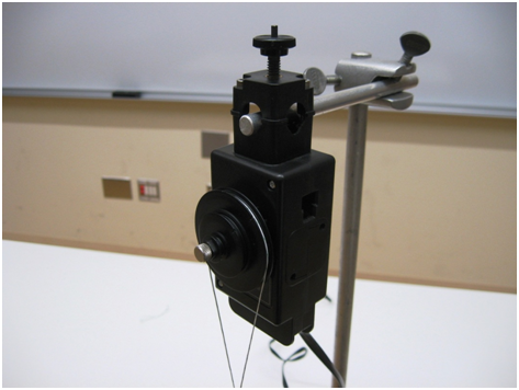
Figure 1
Procedure
Please print the worksheet for this lab. You will need this sheet to record your data.
Data Taking
1
Find the Vernier rotation detector and verify that it is connected to the DIG/SONIC: 2 port on the LabPro interface.
2
To record the data, open the Logger Pro application on your computer. Go to File → Open then go to Probes and Sensors, Rotary Motion Sensor, and finally Rotary Motion Angular High Res. Click the Collect button on the screen and then release the hanging weights and the data is automatically recorded. To change the length of time that data is taken, go to Sampling, which is also Ctrl+M, and then Experiment Length. One may change axes by going to Graph Options and then Axis Options. A sample data run is shown in the Figure 2.
3
Go to the Window menu, choose Table and Select All. Determine from the graph the times when the motion starts and stops. In the table, select the "Time" and "Angle" columns from the starting time down to the point where the motion stops. Copy this information from Logger Pro by using Ctrl+C.
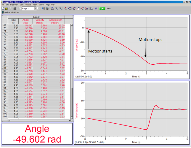
Figure 2
4
Open Excel and paste the data into the Excel spreadsheet.
5
Choose the Chart Wizard, which looks like a bar graph. Select XY (Scatter). For the range choose the θ data, which should be in the second column. Select the Series tab and put in the time, which should be in the first column, as the horizontal values (here called x by Excel even though its the time!) Then hit Finish.
6
Click on the graph and then select the Chart menu. Go to Trendlines. For the Type select Polynomial and for Order put in 2. Click on Options and select Display Equation on Chart. You should now have the function θ(t) that has been the object of so much attention in the lectures.
7
Now change the hanging weights by a small amount and take another data run recording these data in an Excel chart as you did for the first run (add a paper clip or two to the heavier mass side). We will come back to these two data sets in a later section.
Analysis of Data
8
Given the polynomial fits to the two data sets, you should be able to calculate the derivative of θ(t) using the rules for differentiation. You then have the angular velocity as a function of time. Record the coefficients for the function of angular velocity as a function of time from the data sets above for a later comparison.
9
The goal of this next data analysis is to verify that you can get the velocity at any particular time by doing the limit process. Choose a time early in the range of t and call it t1. We want t2 to be a later time at which θ(t) was recorded. Therefore let
There was a certain time interval between data points determined by the apparatus. Let us call this time interval z. Then we can write
where n is the number of intervals between t1 and t2. (Now by changing the integer n we can change the size of Δt.) From the column of θ(t) in the spreadsheet, calculate
with
and the limit as n goes to a small number is the limit as Δt goes to zero.
for n decreasing from some large number to 1. What you are calculating is
10
Plot the results of Equation (10) as a function of n. If everything works as it should, in the limit of Δt approaching zero Equation (10) should approach the value for ω(t1) you get by putting t = t1
in the function ω(t) obtained by taking the derivative of θ(t) in step 6.
11
Using your Excel data taken earlier, calculate this limiting process for five different time intervals in each of your two data sets.
-
aTo do this, copy your data onto a new worksheet and then using the time and angle data, calculate the difference in angle divided by the difference in time, for data separated by an integral number of bins, forn = 5, 4, 3, 2, 1.
-
bFor each of these time intervals, make a scatter plot of the slope of the angle versus time data as a function of the number n and using a linear trendline, find then = 0intercept of these curves.
-
cEnter these intercept values, along with the time values in Table 1 (column titled intercept).
-
dNow compare these results to the values of the angular velocity that come from your fit of the derivative above evaluated at these times. Enter these values into the data table as well (column ω1(n)).
-
eHow do they compare?
12
Repeat this process for the second set of data with a different set of hanging weights (add a paper clip or two to the heavier mass side) and enter that data into Table 2.
Checking the Acceleration
The acceleration of the hanging weight should be proportional to the angular acceleration of the disk.1
Using the polynomial fit and differentiating twice you should be able to calculate the experimental value of the angular acceleration.
2
With a timer and a ruler, measure and time the weight as it travels a known distance and from this calculate its acceleration.
3
You should verify that for both sets of data, a = αR
where R is the radius of the disk.
4
Do your results agree with this prediction within your experimental errors?