
Simple Pendulum
Introduction
A swinging pendulum keeps a very regular beat. It is so regular, in fact, that for many years the pendulum was the heart of clocks used in astronomical measurements at the Greenwich Observatory. Refer to Figure 2 for some terminology of simple harmonic motion.The Pendulum
A simple pendulum is just a mass tied to the end of a string that is fixed to an attachment point so that the mass is free to swing. If we look at this system in more detail, we see that while the mass is swinging, it is subject to a changing force of gravity and the tension in the supporting string. (See Figure 1 below.)
Figure 1
ω =
.
In trying to understand what properties of the simple pendulum result in it having a very regular beat, or period (the time, T, for one complete cycle), there are at least three things you could change about a pendulum.
 |
|
-
•the amplitude of the pendulum swing
-
•the length of the pendulum, measured from the center of the pendulum bob to the point of support
-
•the mass of the pendulum bob
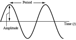
Figure 2
Objectives
-
1To measure the period of a pendulum as a function of the amplitude of its motion.
-
2To measure the period of a pendulum as a function of the length of the pendulum.
-
3To measure the period of a pendulum as a function of the mass of the pendulum.
-
4To observe that energy is being conserved in the simple pendulum system.
Apparatus
- Computer
- LabPro Interface Box
- Logger Pro Software
- Vernier/PASCO Rotary Motion Sensor (RMS)
- String with a small washer to be used to adjust the pendulum length
- Hooked masses of 100 g, 200 g
- Meterstick
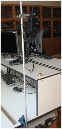
Figure 3
Procedure
Please print the worksheet for this lab. You will need this sheet to record your data.
A: Setup
1
Make a pendulum by using a 75 cm length of string attached to a mass. (Note: To adjust the length of the pendulum you will need to lift the weight slightly to reduce the tension in the string and then slide the washer up or down the string as needed.) Hold the string in your hand and let the mass swing. Observing only with your eyes, does the period depend on the length of the string? Does the period depend on the amplitude of the swing?
2
Try a different mass on your string. Does the period seem to depend on the mass?
3
Now hang the 200 g hooked mass on the end of the string of step 1. Hang the string from the largest diameter pulley on the rotary motion sensor (RMS). The length of the pendulum is the distance from the axis of the pulley to the center of the mass. The pendulum length should be about 75 cm.
4
Verify that the rotary motion sensor is connected to the DIG/SONIC 1 port of the LabPro interface unit.
5
Prepare the computer for data collection.
-
aDouble click on the Logger Pro icon to start the program.
-
bChoose Open from the File menu.
-
cOpen the folder named "probes and sensors", then "rotary motion sensor" and then finally "rotary motion sensor angular Hi-Res".
-
dSelecting this option then displays a graph of position (angle) vs. time as well as the data table. (Note:θ° = 360°/rev × θ rev.)
-
eTo acquire data, let the mass hang stationary and zero the motion sensor by pressing the 0 button next to the Collect Data button at the top of the tool bar. Once the sensor has been zeroed, then start the pendulum swinging and then click on the Collect Data button.
-
fAfter taking data, you can always repeat a run by clicking on the Collect Data button.
Note that sometimes despite the zeroing of the sensor, the data is not centered on zero angle. This is not a problem since we will be using the Logger Pro fitting program and this will give us the value of the observed offset. (See Figure 4 below.)
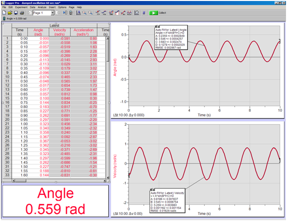
Figure 4
6
Now you can perform a trial measurement of the period of your pendulum. Pull the mass to the side about 10° from vertical and release. Click the Collect Data button and collect data for ten seconds or so.
7
The table window on the left of the screen is a spreadsheet containing the measured values for time and position (θ). Use from four to six complete cycles and record the elapsed time between the start of the first chosen cycle and the end of the final chosen cycle in order to determine the period for this configuration of the pendulum.
B: Determining How Period Depends on Amplitude
1
Now measure the period for five different amplitudes. Use a range of amplitudes, from about 5° to about 30°. Each time, note the initial and final amplitudes and record the average amplitude for the data set.
2
Repeat part A, step 7 for each different amplitude. Record the data in a data table.
C: Determining How Period Depends on Length
1
Use the method you learned above to investigate the effect of changing pendulum length on the period. Use the 200 g mass and a consistent initial amplitude of about 20° for each trial. Vary the pendulum length in steps of 10 cm, from 0.6 m to 1.0 m.
2
Repeat part A, step 7 for each length. Construct a data table and record all the data in this table. Measure the pendulum length from the RMS pulley axis to the middle of the mass.
D: Determining How Period Depends on Mass
1
Use the two masses to determine if the period is affected by changing the mass. Measure the period of the pendulum constructed with each mass, taking care to keep the distance from the ring stand rod to the center of the mass the same each time, as well as keeping the amplitude the same.
2
Repeat part A, step 7 for each mass (100 g and 200 g), using an amplitude of about 20°. Record all the data in a data table.
E: Using Excel
1
Use Excel to plot a graph of pendulum period vs. amplitude in degrees. Scale each axis from the origin (0, 0). Does the period depend on amplitude? Explain.
2
Use Excel to plot a graph of pendulum period, T vs. length, l. Scale each axis from the origin (0, 0). Does the period appear to depend on length?
3
Use Excel to plot the pendulum period vs. mass. Scale each axis from the origin (0, 0). Does the period appear to depend on mass? Do you have enough data to answer conclusively?
4
To examine more carefully how the period, T, depends on the pendulum length, l, use Excel to create the following two additional graphs of the same data: T2 vs. l and T vs. l2. Of the three period-length graphs, which is closest to a direct proportion; that is, which plot is most nearly a straight line that goes through the origin?
5
Using Newton's laws, we can show that for the small oscillations of a simple pendulum, the period, T, is related to the length, l, and free-fall acceleration, g, by T = 2π
.
Do any of your graphs support this relationship?
|
|
6
From your graph of T2 vs. l determine a value for g.
Try a different method to study how the period of a pendulum depends on the amplitude.
On the menu bar, click on Experiment and then Data Collection. In the window, set the experiment length to 60 sec and the sampling speed to 10 samples/sec. Start the pendulum swinging with a fairly large amplitude. Start data collection with an initial amplitude near 45° and allow data collection to continue for a minute or two. Restart the oscillations if you don't get the motion of the pendulum in the plane perpendicular to the axis of the pulley on the sensor. The amplitude of the swing will gradually decrease and you can see how the period changes with amplitude. (See Figure 5 below.)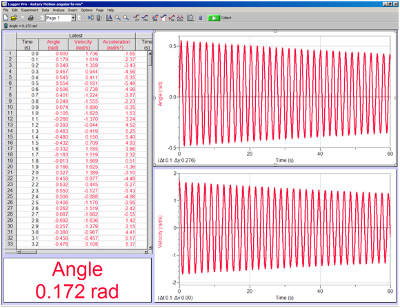
Figure 5
7
Determine the period for four intervals spread over the total time, each containing four or five oscillations.
-
aOn the menu bar click on Analyze → Curve Fit.
-
bChoose theA sin(B · t + C) + Dformula and click on the Try It button and then click OK.
-
cChoose a region of fit by left-clicking the cursor at the desired lower channel, then drag the pointer to the desired upper channel and release the "click."
-
dIf the fit looks reasonable, enter your data into Table 4. Be sure to use the labels Average Amplitude (in degrees) and Average Period (in seconds),T (sec) =
=2 π ω
.2 π B
F: Studying Energy Conservation
1
Prepare the computer again for data logging. This time we wish to take a short 10 second run with a small amplitude displacement to study how energy is conserved in this system.
-
aTo acquire data, start the pendulum swinging and then click on the Collect Data button once again.
-
bAfter taking data, you can always repeat a run by clicking on the Collect Data button.
2
Collect data for an initial amplitude of 10°–15° over several complete swing cycles.
-
aOn the menu bar, click on Analyze → Curve Fit for the angle versus time data you have just taken.
-
bChoose theA sin(B · t + C) + Dwith the following steps.
-
cDouble click on one of the numbers, excluding the very top and bottom numbers, on the vertical scale of the graph window and select Axes Option and set scaling to "Autoscale" to expand the data on the screen. With the equationy − D = A sin(B · t + C),make a rescaled graph which oscillates abouty = 0with the following steps.
-
iClick Data → New Calculated Column and give the name "theta, units = rev".
-
iiConstruct equation by clicking on Position(Angle) in the variables box and add the value of "–D" from the fit you just completed.
-
iiiClick on the Options tab on the top of the box and pick a color.
-
ivClick Done when finished.
-
vGo to Insert click on the graph (graph plotting theta/time is displayed).
-
-
dNow do the same procedure for the angular velocity data that has been recorded by Logger Pro. Once again you will want to fit this angular velocity data toA sin(B · t + C) + Dformula.
3
From these two data sets you can now calculate the kinetic energy and the gravitation potential energy of the swinging mass as a function of time. Find the total mechanical energy of the system at an angle of zero and for the maximum angle that the mass makes during its swing. How do these two values compare?