
Waves on Strings
Objectives
-
•to explore various properties of waves traveling along a Slinky
-
•to explore various properties of standing waves on a string
Equipment
- large Slinky
- stopwatch
- 30-m measuring tape
- spring scale
- PASCO vibrator powered by the variable frequency function generator
-
string of a known linear density (1.35 × 10⁻⁴ kg/m)
- set of masses from 50 g to 1000 g
- 50-g weight hanger
- pulley
- meter stick
Introduction and Theory
Waves are one of the most important concepts in physics. They exist as waves on strings, sound in air and in solids, light, radio waves, microwaves, x-rays, and matter waves. Matter waves are the basis of the advanced field theory called quantum mechanics. All of these waves share much in common. A stretched string will be a very visual demonstration of wave phenomena in general. In this lab we are going to study how waves travel on strings similar to the ones in many stringed musical instruments such as violin, guitar, and piano. In contrast to the sound waves which are longitudinal, waves on a string are transverse. This means that the displacement of the wave is perpendicular to its direction of propagation.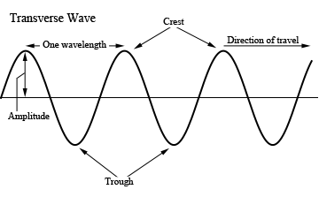
Figure 1
( 1 )
ν =
 |
|
 |
| m |
| l |
 |
( 2 )
ν =
.
|
|
( 3 )
x = x0 cos(2πft).
( 4 )
y = y0 sin 2π
ft ±
|
| x |
| λ |
|
( 5 )
ν = fλ.
ν =
|
|
ν = fλ.
we can describe the wavelength as
( 6 )
λ =
| 1 |
| f |
|
|
T = Fg = Mg,
the expression for the wavelength becomes:
( 7 )
λ =
.
| 1 |
| f |
|
|
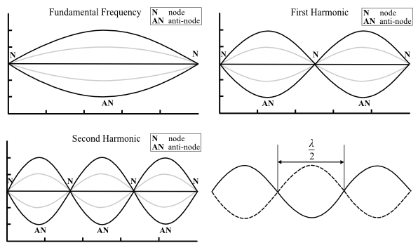
Figure 2: standing waves on a string with fixed endpoints
( 8 )
L = n
|
| λ |
| 2 |
|
Procedure
Please print the worksheet for this lab. You will need this sheet to record your data.
Part A: Traveling waves on a Slinky
Caution:
Handle the Slinky very carefully to avoid any possible permanent damage or distortion to the Slinky.
Handle the Slinky very carefully to avoid any possible permanent damage or distortion to the Slinky.
Part A.1
1
On the Lab 9 Worksheet, Part A, record the mass of the Slinky, which is given on the attached label.
2
The Slinky acts like a string for the purpose of propagation of transverse waves. Two lab partners should stretch the Slinky out to a length of about 20 ft in the hallway. The tile squares are 1 ft2. Have the Slinky rest on the floor for much of its length.
3
One partner should launch a pulse, which will travel down the Slinky while the other partner measures the time it takes for the pulse to reach the opposite end. In order to get the hang of this, you will need to make several trials. Assess the average travel time from three good runs. Record it in the Lab 9 Worksheet, Table 1. You will need to find the uncertainty in time using the statistics function in GA.
4
Use the spring scale provided to measure the tension (in Newtons) in the Slinky.
Part A.2
1
Repeat steps 2-4 from Part A.1 for the Slinky stretched to about 30 ft. Record the time from the three good runs on the Lab 9 Worksheet, Table 2.
Since the Slinky acts like a perfect spring, the time to propagate a wave down the Slinky will be about the same no matter what the length is. Another thing you should notice from this experiment is that the reflected pulse is inverted with respect to the incident pulse. This occurs because the end point is fixed and therefore can't move. You will need to mention these properties in your discussion.
In your Lab report, you will need to calculate the experimental speed of the Slinky and its uncertainty. (Hint: v = L/tave; where L is the length of the stretched Slinky and tave represents the average travel time.) Calculate the theoretical speed using eqn. 1ν =
|
|
Part B: Standing waves on a string
The lab apparatus consists of a string, which is fixed on one end and attached to a weight hanger over a pulley on the other end as shown in fig. 3. The string is driven by a wave generator, which excites the string in a direction perpendicular to the string. The wave driver is like a loudspeaker without the cone that radiates sound. The wave driver is connected to a function generator/power amplifier. The function generator can put out a sine wave of variable frequency and variable amplitude.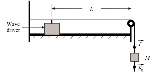
Figure 3: the waves on a string setup
Part B.1. Constant Tension
1
Measure the length between the end supports of the string. Record it on the Lab 9 Worksheet.
2
Put the 200-g mass on the weight holder and tune the function generator to find the resonance condition (standing wave with maximum amplitude) for one anti-node.
3
Calculate the tension in the string. The mass of the weight holder is 50 g. (Hint: refer to the force diagram in figure 3.) Remember to include the mass of the weight holder.
4
On the Lab 9 Worksheet, Table 3, record the resonant frequency for n = 1.
5
Now tune the function generator to higher frequencies and find resonant frequencies up to n = 6.
6
In the Lab report, you will need to calculate the wave velocity for each case to check if it stays constant.
7
In GA, create two manual columns of 'frequency' and 'number of anti-nodes'. Record your data from the Lab 9 Worksheet. Plot the graph frequency f vs. number of anti-nodes n. Apply linear fit to the graph. From the slope of the regression line, compute the experimental wave velocity and its uncertainty. Calculate the theoretical value of wave velocity based on eqn. 1ν =
|
|
8
Upload a file with your graphs. Do a print screen and save the graphs as a file with a maximum size of 1 MB. Print the graphs for your TA to sign, and for your reference.
Part B.2. Constant Wavelength
Now you will make a series of measurements for n = 1 varying the tension in the string.1
Measure the length between the end supports of the string, in case it got changed. Record it on the Lab 9 Worksheet.
2
Place a 100-g mass on the weight holder. Find the resonance frequency for n = 1. Record it in the Lab 9 Worksheet, Table 4. Using masses in the range from 100 g to 1000 g (including the mass of the weight holder), vary the tension in the string. For each new value of tension find a resonance frequency for n = 1. Keep recording data on the Lab 9 Worksheet, Table 4.
3
Create new manual columns in GA. Label them mass and frequency. Record your data from the Worksheet into GA. Create two calculated columns: Tension and square root of Tension - Sqrt (Tension). Plot the graph frequency vs. Sqrt (Tension). Apply linear fit and record the slope and its uncertainty on the Lab 9 Worksheet.
4
Calculate the expected theoretical value of the slope that can be derived from eqn. 5ν = fλ.
and eqn. 7λ =
.
| 1 |
| f |
|
|
5
Using the value of the slope, calculate the experimental value of the linear density of the string. Compare it to the theoretical value provided in the lab manual by calculating the percent discrepancy.
Discussion Questions
Does the experiment support the theory stating thatν =
?
|
|