
Hooke's Law and Simple Harmonic Motion
Objective
-
•to measure the spring constant of the springs using Hooke's Law
-
•to explore the static properties of springy objects and springs, connected in series and parallel
-
•to study the simple harmonic oscillator constructed from springs and masses
-
•to verify that the period of the SHM is proportional to the square root of the mass and independent of the amplitude
-
•to measure the dynamic spring constant
-
•to verify the conservation of energy law
Equipment
Part I:
-
•two nearly identical springs
-
•long rubber band
-
•support stand with a meter stick
-
•50 g mass hanger
-
•set of masses from 100 g up to 600 g
-
•balance scale
-
•Science Workshop Interface with force sensor and rotational motion detector used as a linear sensor
Part II:
-
•collision cart of a known mass on a horizontal dynamics track oscillating by the means of springs in parallel
-
•motion sensor and photogate connected to the Science Workshop interface
-
•non-linear springy objects (rubber bands)
-
•two rectangular weights of ~0.5 kg each to change the mass of the system
Introduction and Theory
Hooke's Law
Elastic force occurs in the spring when the spring is being stretched/compressed or deformed (Δx) by the external force. Elastic force acts in the opposite direction of the external force. It tries to bring the deformed end of the spring to the original (equilibrium) position. See fig. 1.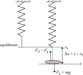
Figure 1
( 1 )
Fel = −kΔx
Fel = −kΔx
indicates that the elastic force and stretch act in the opposite direction.
Simple Harmonic Motion
If the hanging mass is displaced from the equilibrium position and released, then simple harmonic motion (SHM) will occur. SHM means that position changes with a sinusoidal dependence on time.( 2 )
x = Xmax cos(ωt)
( 3 )
v = −Xmaxω sin(ωt)
( 4 )
a = −Xmaxω2 cos(ωt)
x = Xmax cos(ωt)
, 4a = −Xmaxω2 cos(ωt)
and 1Fel = −kΔx
into Newton's Second Law, one can derive the equation for the angular resonant frequency of the oscillating system:
( 5 )
ω =
 |
|
radians per second = rad/s.
The natural resonant frequency of the oscillator can be changed by changing either the spring constant or the oscillating mass. Using a stiffer spring would increase the frequency of the oscillating system. Adding mass to the system would decrease its resonant frequency.
Two other important characteristics of the oscillation system are period (T) and linear frequency (f). The period of the oscillations is the time it takes an object to complete one oscillation. Linear frequency is the number of the oscillations per one second. The period is inversely proportional to the linear frequency.
( 6 )
T =
| 1 |
| f |
( 7 )
ω = 2πf =
| 2π |
| T |
Energy
In order for the oscillation to occur, the energy has to be transferred into the system. When an object gets displaced out of equilibrium, then elastic potential energy is being stored in the system. After the object is released, the potential energy transforms into kinetic energy and back. In the harmonic oscillator, there is a continuous swapping back and forth between potential and kinetic energy. For an oscillating spring, its potential energy (Ep) at any instant of time equals the work (W) done in stretching the spring to a corresponding displacement x.( 8 )
Ep = W =
kx2
| 1 |
| 2 |
( 9 )
Ek =
mv2.
| 1 |
| 2 |
( 10 )
Ep =
kXmax2
| 1 |
| 2 |
( 11 )
Ek =
kVmax2
| 1 |
| 2 |
Procedure
Please print the worksheet for this lab. You will need this sheet to record your data.
Part I - Hooke's Law
Measurement of a spring constant, method 1
The purpose of this part of the laboratory activity is to find the spring constant of the spring. The spring constant is a coefficient of proportionality between elastic force and displacement, according to Hooke's Law (equation 1Fel = −kΔx
).
1
Hang a spring from the support, add a weight hanger, and measure the initial equilibrium position with the meter stick and record it.
2
Add masses in steps of 100 g up to 600 g and measure the corresponding position.
3
Discuss with your group members the columns that need to be prepared in GA to record the data. Make a draft of a table and check it with your TA. Prepare the columns in GA.
4
Create a new calculated column for the elastic force data (DATA → NEW CALCULATED COLUMN → equation: F = variables "m"*g, where m is in kg).
5
Create a new calculated column for displacement (DATA → NEW CALCULATED COLUMN → equation = variables "position" — initial equilibrium position).
6
Make a plot of force vs. displacement.
7
Record the slope of the graph and its uncertainty in the Lab 8 Worksheet. You will use the value of slope and its uncertainty to find the spring constant and its error.
Measurement of spring constant, method 2
The apparatus setup shown in fig. 2 will be used to find the spring constant in spring 2.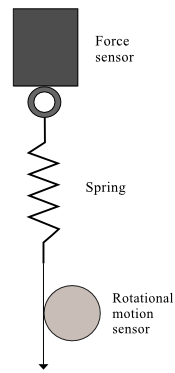
Figure 2: The apparatus setup for the Hooke's Law experiment
1
Open the pre-set experiment file: desktop\pirt-labs\phy 113\PreSetUpFiles\Springs.
2
Before taking the actual data, calibrate the force sensor. Click the "Setup" button in the toolbar. Then click on the force sensor icon and press the "Calibrate Sensors" button. This brings up the calibration panel shown in fig. 3.
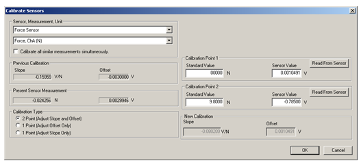
Figure 3: Calibration of force sensor in Data Studio
The "2 Point" option should be selected as the "Calibration Type". With no load on the force sensor, enter 0 in the "Calibration Point 1" standard value window. Push the "Tare" button on the force sensor. This action adjusts the force sensor reading to zero. Press "Read From Sensor" button. Next hang the 1 kg hooked mass on the sensor and type 9.8 in the "Calibration Point 2" standard value window. Click on the "Read From Sensor" button. Click on "OK" to save this calibration. Close the "Calibrate Sensors" and the "Setup" windows. Now you are ready to take the actual measurements of the spring constants.
3
Replace the 1 kg weight with the spring. Attach a piece of string to it. Wrap the string around the large pulley of the rotational motion detector in a counter clockwise direction as depicted in fig. 2. The rotational motion sensor has been calibrated to read the linear distance.
4
Press the "Start" button to initiate the data acquisition. Carefully pull on the string, watching the Force display window. Start releasing the string when the force reaches up to 10 N.
5
Apply the linear fit to the good part of your recording (see fig. 4) which presents elastic force vs displacement graph. The slope of this line gives the spring constant.
6
Record the slope of the Force vs potion graph and its uncertainty in the Lab 8 Worksheet. You will use the value of slope and its uncertainty to find the spring constant and its error.
7
Repeat this procedure for a system of springs in series and in parallel.
8
Record the slope of the Force vs position graph and its uncertainty in the Lab 8 Worksheet. You will use the value of slope and its uncertainty to find the spring constant and its error. In the Discussion section, you will need to compare the value of the spring constants for the system of springs to the value of each spring constant.
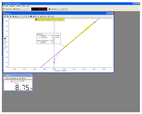
Figure 4: A sample of experiment file in DataStudio
Investigation of nonlinear springy object.
1
In the experimental setup from fig. 2, replace the spring with the long rubber band.
2
Record force vs. position for both down (increasing force) and up (decreasing force) strokes.
3
Use this data to address whether or not the rubber band follows Hooke's Law (equation 1Fel = −kΔx
).
Part II - Simple Harmonic Motion
In this part of the experiment you will verify if the period depends on the amplitude; calculate the resonance frequency and spring constant of a system. You will record the collected data in the Lab 8 Worksheet.1
Setup the experiment as shown on the pictures below. Open the pre-set experiment file: desktop\pirt-labs\phy 113\PreSetUpFiles\SHM.
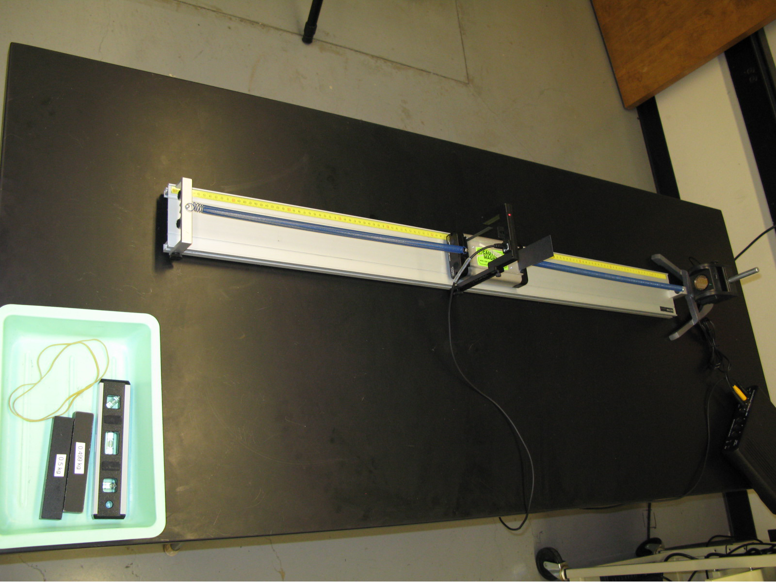
Figure 5
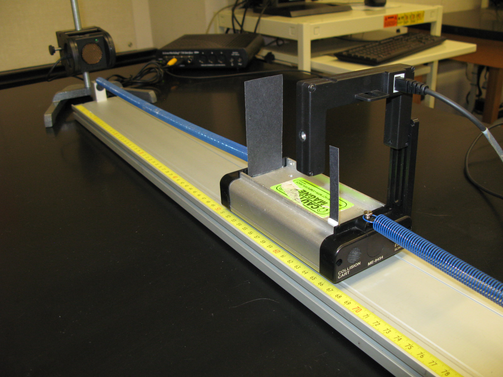
Figure 6
2
With no added mass, measure the period of oscillations for starting amplitudes of 4 cm and 12 cm. Data acquisition will stop automatically after 5 sec. The sample recording is shown in fig. 2. The period is measured by the photogate and recorded in the table 1 to the left of the graph.
3
With no added mass, displace the cart from its equilibrium position about 8 cm and start the recording. Record again the period of oscillations of a cart measured by the photogate. Record all three periods of oscillations in the Lab 8 Worksheet.
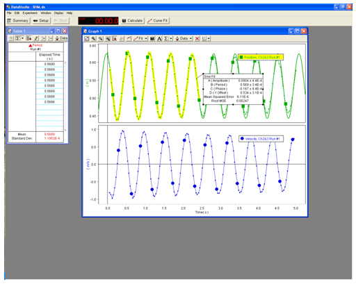
Figure 7: A sample file for SHM experiment in DataStudio
4
Fit the recording of position vs. time to the sine wave. Parameter A is amplitude (maximum displacement) of the oscillations. Parameter B gives you the period of oscillations. You can compare its value to the value of the period measured by photogate. Parameter D — is the equilibrium position. Use parameter B to calculate resonance frequency and spring constant of a system using equations 7ω = 2πf =
and 5| 2π |
| T |
ω =
|
|
5
Fit the recording of velocity vs. time to the sine wave. Record the parameter A — the amplitude (maximum value) of the velocity vs time graph.
| π |
| 2 |
( 12 )
%loss =
· 100%
| PEi − KEf |
| PEi |
Relationship between period and mass
This is the part of the experiment where you will verify that the period of the SHM is proportional to the square root of the mass.1
Load the cart with heavy masses (one at a time) and measure the period of SHM while keeping the amplitude constant, e.g. 8 cm.
2
Including the data from the previous part of the experiment, you will have three points to make a graph of period vs.  | m |
ω =
|
|
ω = 2πf =
) this graph should be a straight line.
| 2π |
| T |
3
Record the slope of the T vs | m |
4
Use the value of slope and its uncertainty to find the spring constant.
5
Based on the slope of the graph calculate the dynamic spring constant of the system.
Hint: Substituting
-
ω =
2π T
-
ω =
k m
-
=2π T
.k m
-
T =
2π k m