
Free Fall – Concepts
Discussion of Principles
The first part of this document derives the equations necessary for the lab from the definitions of average velocity and average acceleration in the manner of PY205N. Following this is a section that derives the same equations from the momentum principle in the manner of 205M.
Derivation Using Average Velocity and Acceleration – PY205N
This discussion relates to the motion of an object under the influence of a uniform acceleration (such as being in free fall under the influence of gravity). In the following derivations, downward is treated as the positive y-direction, but this is simply a convention. Either direction could be positive so long as all upward-pointing vectors have the opposite sign of the downward-pointing ones (in other words, just be consistent).Average Velocity and Average Acceleration
Consider an object at position y1 at some initial time, t1. At a later time, t2, the object is at location y2. The average velocityv12
for this object as it travels between these two points will be
Similarly, the average velocity v23
during the next time interval (that is, between the instants t2 and t3) is
If the acceleration is uniform or constant, the instantaneous velocity at exactly the midpoint of the time interval is the average velocity. Even if the acceleration were not uniform, this would be a close approximation if the interval of time were short. So v23
would occur at the midpoint of the time interval given by
With these two average velocities and times, we can calculate an average acceleration a
as
where Δv and Δt denote the change in velocity and time, respectively.
Motion Graphs
For an object moving with constant velocity, a plot of distance versus time would be a straight line with a constant slope like the graph in Figure 1a below. Since distance is plotted on the vertical axis and time is plotted on the horizontal axis, the slope is| Δ (Distance) |
| Δ (Time) |
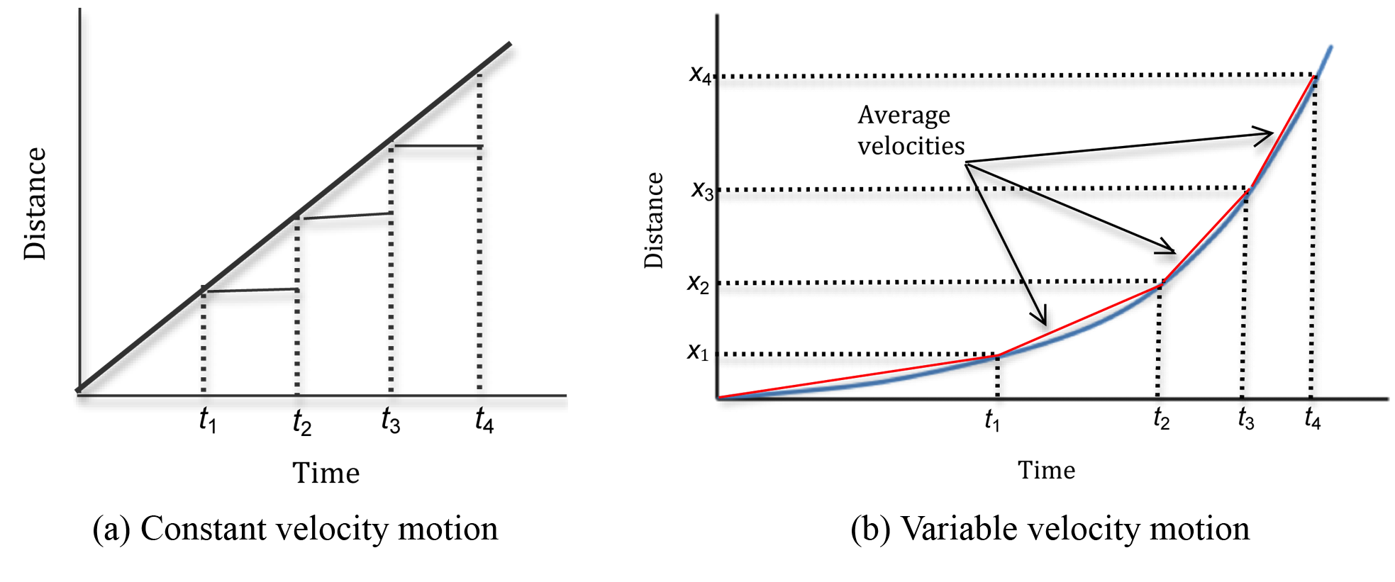
Figure 1: Plots of distance versus time
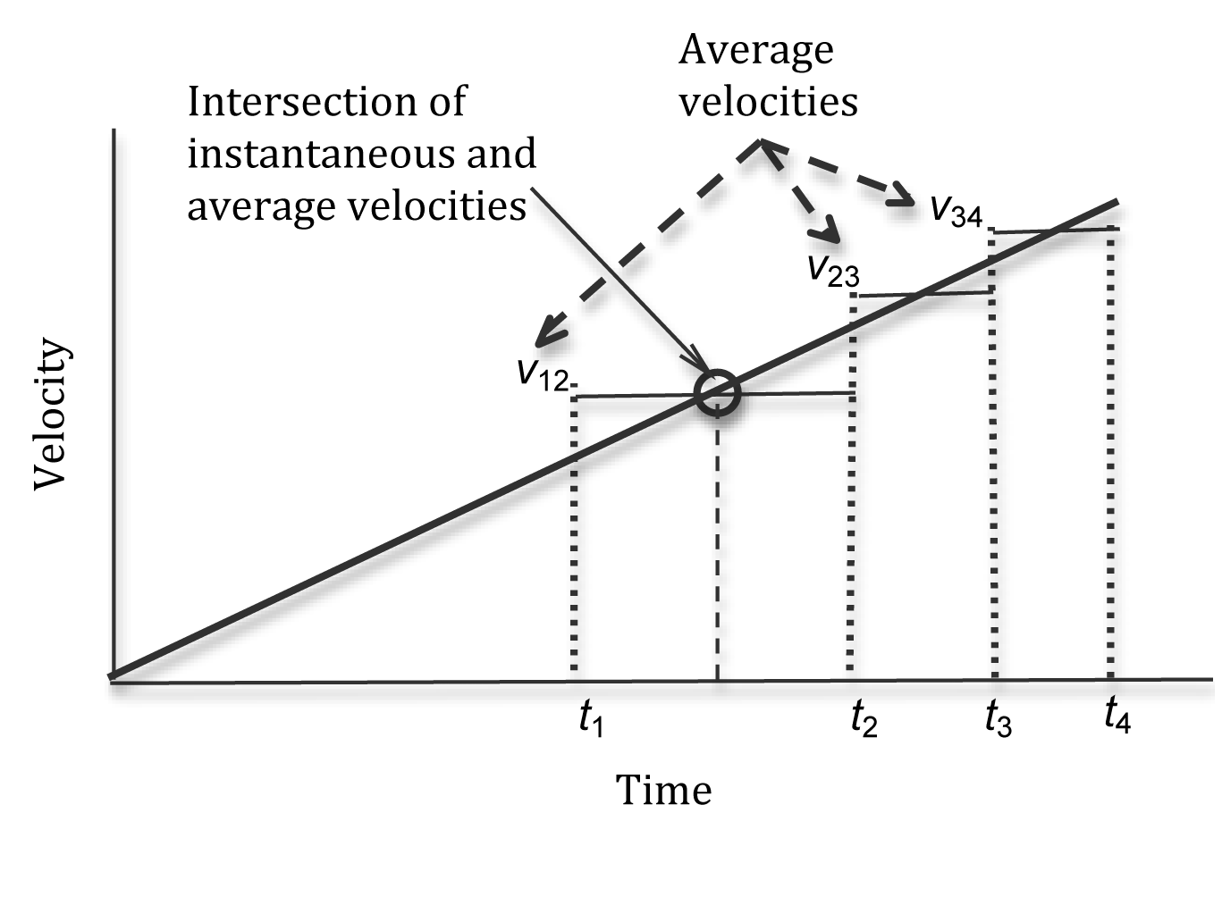
Figure 2: Graph showing instantaneous and average velocities
Kinematic Equations
The kinematic equations are derived from the definitions of average velocity and acceleration discussed above for a uniformly accelerating object. These equations provide a useful way to evaluate the motion of an object moving with constant acceleration. For one-dimensional motion, the kinematics equations are where vi and vf are the initial and final velocities when the object is at positions xi and xf respectively, Δt is the elapsed time, and a is the constant acceleration for this motion.Free Fall
With the object being released from rest, vi = 0. The acceleration is equal to g in the downward direction (defined as positive in the beginning of this discussion), and the total displacement is downward and equal to the height from which the object was dropped (assuming the object falls all the way to the ground). Making these substitutions into equation 6 yields the following form which is the equation that relates drop height to drop time and the acceleration due to gravity.
This is the equation that you will use most often during this lab.
Derivation Using the Momentum Principle – 205M
For an object experiencing free fall, the only force acting on it is the force of gravity. (For this experiment we will neglact the force of air resistance.) Near the surface of the Earth, the force of gravity can be approximated, byFEarth =
0, −mg, 0
,
where  |
 |
g ≈ 9.81 m/s2.
Thus, from the momentum principle, we can determine the effects of this force.
From here we will consider only the y-components of the equations, as the other components have no net force. We will also replace p with mv, taking γ = 1 for the speeds the object will attain.
Since the object's mass appears in every term, it can be cancelled out, leaving an equation that exactly matches equation 5vf = vi + aΔt
above when the acceleration is equal to g in the downward direction.
Subtracting vi from both sides of the equation yields
and we see that the left side is the definition of vave. Now consider the position update formula.
Since equation 13 showed that the average velocity can be expressed as −
gΔt
, equation 14 can be rewritten with this substituted for vave. The total displacement Δr is downward and equal to the height above the ground at which the object started (assuming the object falls all the way to the ground).
This is identical to equation 8| 1 |
| 2 |
h =
g(Δt)2
, derived from kinematic principles.
| 1 |
| 2 |
This is the equation that you will use most often during this lab.