Introduction to the Oscilloscope and RC Circuits

Introduction

This experiment will lead you through the steps on using an oscilloscope to measure the output of a DC power supply and the output of a function generator and then to utilize the oscilloscope to measure the time dependent properties of a simple RC circuit. This experiment should give you some practical experience in the use of the equipment that will be used in later experiments. Much of the theory has been eliminated, but if you require some background on the equipment, any electronics manual or textbook will provide ample information. Your instructor is also an excellent source of information. Do not hesitate to ask for help if needed. Before starting the lab, we would like to review the principles involved with analyzing the transient response behavior of an RC circuit. This discussion follows closely the discussion in many textbooks that discuss the charging and discharging of a capacitor. First, from our earlier lab using resistors in a simple DC circuit, we saw that the voltage across a resistor is proportional to the current flowing through the resistor and the value of its resistance.

( 1 )

V_R = IR

Further, we also have found that the voltage across a capacitor in a simple circuit is given by:

( 2 )

V_C =

If we now form a simple circuit using a battery, a capacitor, a resistor and a switch, as shown in the figure, we can analyze the voltages and currents flowing in the circuit as a function of time as we move the switch from one position to another.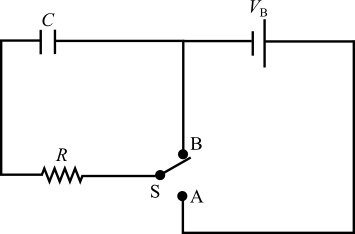

A switch S is located at the middle of a vertical line which can connect to either A or B. The circuit as shown is connected to point B which is above point A. When connected to B, there is a series circuit consisting of a capacitor and a resistor to the left side. The capacitor is labeled C and the resistor is labeled R. When the switch is connected to A, the same capacitor and resistor is also connected to a battery in series. The battery is labeled V_B. The negative terminal of the battery is connected to one side of the capacitor and the positive terminal is connected to the point A.

Figure 1: RC Circuit

RC Circuits - Charging

We will start off considering what happens when we move the switch from position B to position A. Moving the switch in this way connects the battery to the capacitor and resistor network forming a complete circuit which allows charge to flow onto the capacitor. The voltages across the individual circuit elements must satisfy the rules governing the addition of potentials in a circuit and from these we know that:

( 3 )

V_B = V_R + V_C = IR +

R +

In a later math course, you will learn how to solve such linear differential equations; however, this particular equation can be solved by simple integration. (See if you can solve this equation to find the expression for q(t) below.) The solution for q(t) is:

( 4 )

q(t) = q_max(1 − e^−t/RC) = CV_B(1 − e^−t/RC)

where q(t) represents the charge on the capacitor at any particular time, t, after the switch position has changed and with RC representing the characteristic time, τ, for charging the capacitor in this circuit. We can use this result for the charge on the capacitor to now find the current flowing in the circuit as a function of time by taking the derivative of q with respect to t. Doing that we find that the current flowing in the circuit, I(t), is:

( 5 )

I(t) =

V_B

e^−t/RC.

There are two figures here. On the left side, a coordinate plane has the horizontal axis labeled t and the vertical axis labeled q(t). A concave down and increasing curve starts at the origin and reaches the maximum value CV_B asymptotically. On the right side, a coordinate plane has the horizontal axis labeled t and the vertical axis labeled I(t). A curve starts at the maximum value V_B/R at t = 0 and decays exponentially as t approaches infinity.

Figure 2: Charging a Capacitor

RC Circuits - Discharging

After waiting a long period of time (in principle forever, but in practice after only several time constants) the current in the circuit above will have gone to zero and the charge on the capacitor will have reached its maximum value. If at this time, we now switch the position of the switch back to position B, we will initiate the discharging of the capacitor through the series resistor. In this case the rules for adding potentials in a circuit yields:

( 6 )

0 = V_R + V_C =

R +

Again this equation can be solved by integration, and in so doing we find that the charge as a function of time for the discharge of the capacitor behaves as:

( 7 )

q(t) = q_maxe^−t/RC

and the current flowing in the circuit is given by:

( 8 )

I(t) =

−q_max

e^−t/RC.

Note that

q_max = CV_B.

There are two figures here. On the left side, a coordinate plane has the horizontal axis labeled t and the vertical axis labeled q(t). A curve starts at the maximum value q_max at t = 0 and decays exponentially as t approaches infinity. On the right side, a coordinate plane has the horizontal axis labeled t and the vertical axis labeled I(t). A concave down and increasing curve starts in the negative vertical axis at the value -q_max/tau and approaches the positive horizontal axis asymptotically.

Figure 3: Discharging a Capacitor

Objective

In this lab, we will build the simple series RC circuit discussed above, and using the oscilloscope, measure the voltages across the capacitor and the resistor for the charging and discharging of this system. The goal of this lab is to introduce you to the use of an oscilloscope and to use this instrument to observe and measure the transient response of this simple RC circuit as it is being charged and discharged.

Apparatus

Oscilloscope
Function generator
0-40 volt power supply
Circuit box
Multimeter
Miscellaneous banana lead wires

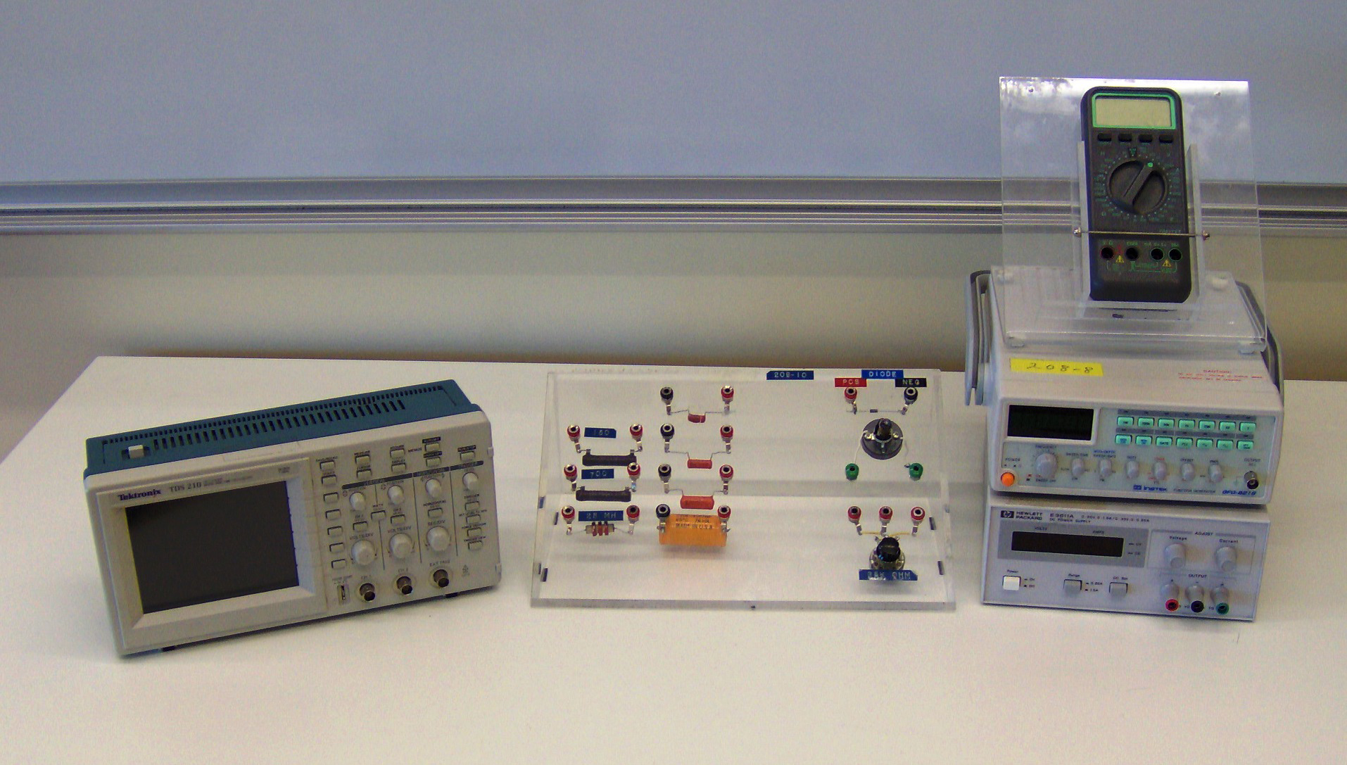
Figure 4: Equipment

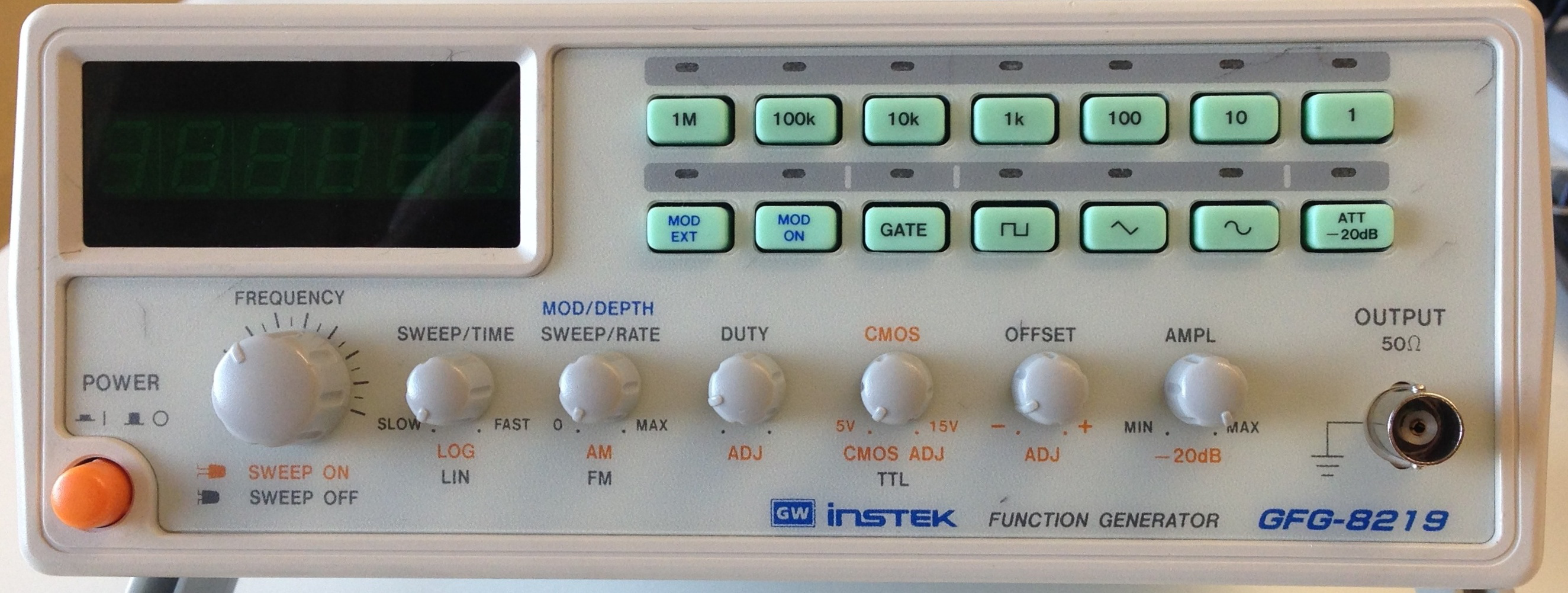
This is an image of the front side of the signal generator. It has a screen and various knobs and an output channel.

Figure 5: Signal Generator

Caution:
Please, be careful in handling all of the equipment in this laboratory. The equipment is expensive and can be easily damaged if misused.

This is an image of the front side of the oscilloscope. It has a screen and various knobs and input channels.

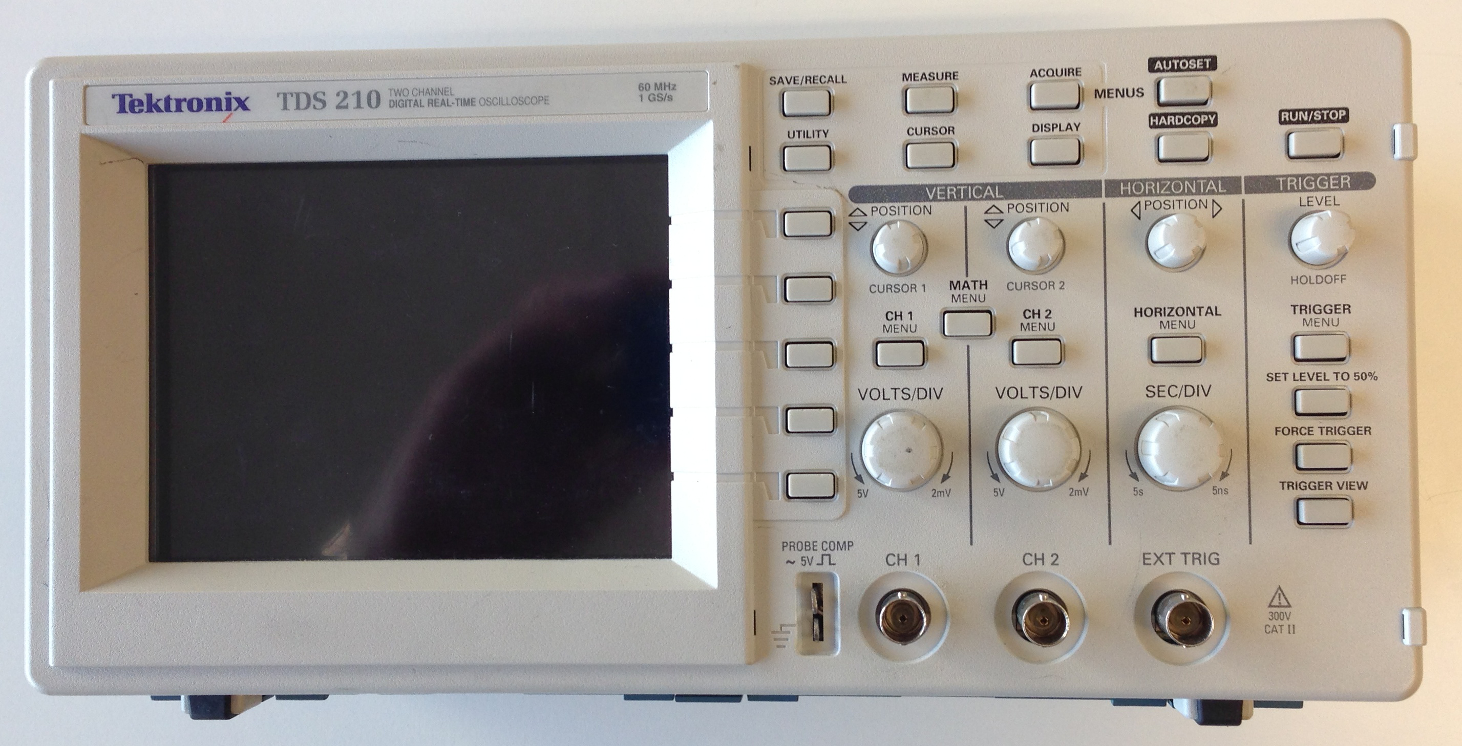
Figure 6: Oscilloscope

Procedure

Please print the worksheet for this lab. You will need this sheet to record your data.

Oscilloscope and Power Supply

Begin by locating the ON/OFF button on top of the oscilloscope. Press this button. The front screen should light up. The oscilloscope will then conduct a self-test to verify the instrument is operating correctly. Wait for the confirmation that everything is OK before proceeding.

It is always a good idea to check the settings of an oscilloscope before beginning any measurements. The following is the set-up procedure to prepare the oscilloscope for the measurements in this laboratory experiment. Most of these settings are probably already preset. Just verify the settings to be sure. The oscilloscope will always reset to the previous settings (the settings that were on the oscilloscope when it was turned off).

Check oscilloscope settings.

a
Press the DISPLAY button. The settings (shown on the right edge of the screen) should be:
- •
  Type [Vectors]
- •
  Persist [Off]
- •
  Format [YT]
- •
  Contrast Increase (Adjustable as needed)
- •
  Contrast Decrease (Adjustable as needed).
  - •
    NOTE: If the intensity is OK, skip this step.

b
Press the TRIGGER MENU button. On the right side of the oscilloscope screen, there are five sections controlled by the five buttons to the right of these sections.
- •
  Video [Edge]
- •
  Slope [rising]
- •
  Source [CH 1]
- •
  Mode [Auto]
- •
  Coupling [DC]
If the settings are not preset to these values, press (once) the button located to the right of the section, next to the scope screen.
c
Press the CH 1 MENU button. The four sections (in the same location as the five sections in part a above, should be set to the following.
- •
  Coupling [DC]
- •
  BW Limit [OFF]
- •
  Volts/Div [Coarse]
- •
  Probe [1x]
d
Press the HORIZONTAL MENU button. The following are the sections that should be selected.
- •
  [Main]
- •
  Trig knob [Level]
e
Press the MEASURE button. The five sections should be set to the following.
- •
  Source [Type]
- •
  CH 1 [Freq]
- •
  CH 1 [Period]
- •
  CH 1 [Pk - Pk]
- •
  CH 1 [Cyc RMS]
f
Locate the VOLTS/DIV knob for CH 1 and adjust it until 2.00 V is displayed on the lower left of the oscilloscope screen.
g
The MEASURE DISPLAY mode should remain on your screen while performing all of your measurements.

You are now ready to set the controls on the power supply in order to get an output to observe on the oscilloscope.

Caution:
Follow these steps carefully.

a
Below the display, you will find three buttons/switches, the leftmost is the POWER switch, then the Range switch, and then the CC Set button.
b
Make sure the power supply On/Off switch is set to Off.
c
On the right side of the power supply, there are two knobs, the Voltage and the Current knob.
d
Rotate both the Voltage and the Current knobs fully counterclockwise (while the power supply is still off).
e
Turn the power supply on.
f
You should see an LED display on the left side of the power supply. The left half of the display shows the voltage, the right half of the display shows the current (in amps).
g
Press the Range button down.
h
Hold the CC Set button down and, at the same time, rotate the Current knob clockwise until the current display reads 0.25 A. This will be the maximum current available from the power supply. Release the CC Set button. Now the display should read zero (0) for the current.

Do not change this setting for the rest of the experiment.

i
The Voltage knob may now be used to vary the output voltage from the power supply.

You shall now do some actual measurements with the oscilloscope.

Check that the VOLTS/DIV setting on the scope is 2.00 V. Connect the output of the power supply (+) and (–) to the CH 1 input of the oscilloscope with the BNC-banana cables. Increase the output voltage of the power supply and see if there is correlation between the power supply output meter reading and the oscilloscope display. Observe the movement of the trace and the reading on the Cyc RMS on the right section of the screen. Reverse the leads on the power supply. Sketch the waveform using the screen template and the Paint program and upload.

Disconnect the power supply and place it aside.

Oscilloscope and Function Generator

You will now use a function generator to produce a signal on the oscilloscope. In order to prepare the generator for use, preset the control as follows.

a
Press the POWER button (orange button on the lower left side).
b
Press the [1k] button on the top row of green buttons.
c
Press the [sine wave] button on the second row of green buttons.
d
Adjust the FREQUENCY control until a reading of 1.500 is displayed on the generator digital readout.
e
The MOD ON and MOD EXT lights should be off.
f
Rotate the AMPL knob clockwise about 1/2 turn. This should produce an output of about 10 volts.

Determine Voltage and Frequency: Method 1

The oscilloscope VOLTS/DIV and SEC/DIV settings should be the following.

•
VOLTS/DIV: 2.00 V
•
SEC/DIV: 250 μs (This setting may be checked by looking at the bottom of the screen [after the symbol M].)

Using the two BNC-banana cables connect the OUTPUT of the function generator to CH 1 of the oscilloscope. Adjust the AMPL(itude) control of the function generator in order to display a 2-3 division waveform on the screen. Note as you adjust the AMPL, the section on the right side (Pk-Pk) of the oscilloscope is reading the peak-to-peak voltage of the waveform on the screen.

Determine the frequency of the sine wave by using the value of the SEC/DIV shown on the screen and counting the cycles of the waveform (your TA will discuss this in more detail during his lab presentation).

•

f =
1
p
(Hz)
•

f = frequency
•
p = the period of the sine wave (number of divisions × SEC/DIV)

What is the frequency of the waveform and the voltage of the waveform?

Once again sketch the waveform observed in steps 3 and 4, using the screen template and Paint.

Determine Voltage and Frequency: Cursor Method

Another method to measure the voltage output and the frequency of the generator is the cursor method.

To determine the voltage output, press the CURSOR MENU button. Using the buttons next to the scope screen, set the following selections.

•
Type [Voltage]
•
Source [CH 1]

While on the Voltage setting, two cursors may be moved up and down the oscilloscope screen. Use the two VERTICAL POSITION knobs to move one cursor to the top edge of the waveform on the screen and move the other cursor to the bottom edge of the waveform. The voltage is then determined as the difference between cursor 2 and cursor 1.

What is the voltage reading?

How does it compare with the value in step 5? Which would you say would be a more accurate reading? Explain.

To determine the frequency, press the CURSOR MENU button and using the buttons next to the screen, set the following.

•
Type [Time]
•
Source [CH 1]

While on the Time setting, use the two VERTICAL POSITION knobs to move one cursor to the beginning of one cycle and the other cursor to the beginning of the next cycle. The frequency (and the period) is then determined as the difference between cursor 2 and cursor 1.

What is the frequency reading?

How does it compare with the value in step 5? Which would you say would be a more accurate reading? Explain.

Examine Different Frequencies

Press the [10k] button on the generator. Discuss what happens to the waveform on the scope screen when the generator is set to 10k. Sketch the waveform for that frequency. Be sure to label the sketch.

Press the MEASURE button and you will see that the period and the frequency of the waveform may be read in the sections on the right side of the oscilloscope screen. Take some time to become more familiar with the information displayed on the oscilloscope screen.

Vary the FREQUENCY control and the AMPL control and discuss what happens to the waveform and the readings on side sections of the oscilloscope screen.

Set the output frequency of the function generator to 100 kHz. Adjust the SEC/DIV knob until at least four complete sine waves are visible on the screen. Sketch the waveform.

Switch the function generator to the square wave output, 2 kHz frequency. Compare the frequency output of the generator to the frequency measured with the oscilloscope. Determine the voltage of the waveform and sketch the waveform.

Measuring the Transient Behavior of a Simple RC Circuit

The objective of this experiment is to observe and measure the transient response of a series resistor-capacitor RC circuit. You will also see how to use this to measure and determine the capacitance in such a circuit. The basic unit of capacitance is farad, which is defined as the capacitance necessary to store one coulomb of charge at a potential difference of one volt. The most commonly used units are microfarads

(1 μF = 10⁻⁶ F)

and picofarads

(1 pF = 10⁻¹² F).

The capacitor which you will probably use will be marked with a decimal fraction in which case the units are in μF.

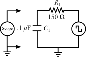
This is a circuit consisting of capacitor .1 micro farad, and a resistor 150 ohms is connected in series to a function generator. The capacitor is labeled C_1 and the resistor is labeled R_1. There is also an oscilloscope which is not yet connected to this circuit.

Figure 7

Finding the Capacitance of a Capacitor

Connect the circuit as shown in Figure 7.

Set the frequency of the function generator to 1 KHz (square wave), the amplitude to maximum.

Set the oscilloscope as described in the Oscilloscope and Power Supply section of this experiment.

Connect CH 1 input of the oscilloscope across the capacitor C in the circuit. Rotate the knobs on the oscilloscope to display the decaying voltage on the capacitor such that the trace touches the top line of the screen and decays to the bottom line of the screen. The trace does not have to fill the screen (horizontally), but it does have to extend over at least 4-5 divisions in order to measure the decay constant.

Record the voltage value of this waveform for at least 10 evenly spaced time intervals from the peak of the wave through its decay to the baseline and record these readings in Table 1. Record these readings as a time and voltage for each reading.

Using this data, record in Table 1 the time and the ln(Voltage).

Plot this as a scatter plot using Excel. Using the trendline feature in Excel, fit this curve with linear function and find the slope and intercept of this curve.

How are these two quantities related to the q_max and RC of this circuit as described in

q(t) = q_maxe^−t/RC?

Disconnect the resistor R from the circuit and measure its resistance. (Note that the internal resistance of the function generator is 50 ohms.)

Calculate the experimental value of the capacitor (C) in the circuit using the formula

τ = RC,

where R is the TOTAL resistance in the circuit. Call it (experimental) C₁. Do not forget the units.

The component value of the capacitor is written on the side of the capacitor. Read and record this value as C₂.

What is the percent error between the experimental value and the component value of the capacitor? Which value do you consider to be more accurate? Why?