
LR, LC, and LRC Circuits
Introduction
In this lab you will be investigating the transient behavior of circuits containing inductors. By transient behavior we are referring to what happens in a circuit when the power is either turned on or off suddenly.LR Circuits
We start by reminding ourselves of the voltage across a resistor (R), a capacitor (C) and an inductor (L). Further, we have defined the current flowing in a circuit in terms of the rate of charge passing a point in the circuit as Combining these four relationships, we can rewrite the value of the voltage across each of these circuit elements in terms of the charge as In an earlier lab, we have already investigated what happens when we charge and discharge a capacitor, so here we will use the same approach to investigate the behavior of a circuit containing an inductor when we turn on and off the power to the circuit.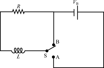
Figure 1
I(t) =
1 − e−(R/L)t
,
| VB |
| R |
 |
 |
τL =
.
| L |
| R |
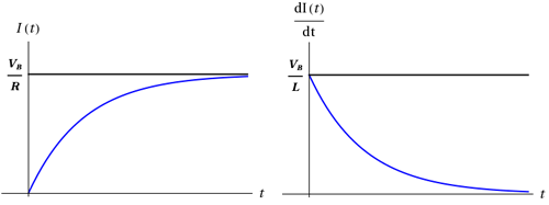
Figure 2
| VB |
| R |
|
| dI |
| dt |
|
VB = VR + VL = IR +
L,
to get the following.
| dI |
| dT |
0 = VR + VL = IR +
L
| dI |
| dt |
τL =
we find
| L |
| R |
( 7 )
I(t) = Ioe−t/τL.
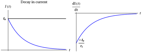
Figure 3
VL =
L and τL =
,
| dI |
| dt |
| L |
| R |
"current rising"
VL = VB e−t/τL
"current falling" VL =
e−t/τL
L =
−Io
e−t/τL
L = −VB e−t/τL
|
| −Io |
| τL |
|
|
|
| R |
| L |
|
|
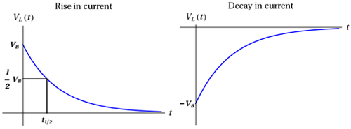
Figure 4
LC Circuits
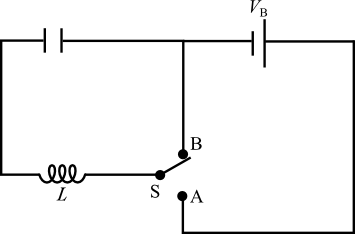
Figure 5
VR = IR
, (2)VC =
, and (3)| q |
| C |
VL =
L
above, we know that the voltage across the capacitor is related to the voltage across the inductor as follows.
| dI |
| dt |
VC =
= VL = −L
| q |
| C |
| dI |
| dt |
| q |
| C |
| d2q |
| dt2 |
q(t) = Ae−(R/2L)t cos(ω' t)
Objective
In this lab you will build an RL and an LC circuit and use the response of these circuits to a time varying voltage that we calculated above to measure the value of the inductance (LR circuit) and the frequency of oscillation of the LC circuit. You will also investigate the effect of the internal resistance in the LC circuit and how that modifies the solution for the charge as a function of time in these circuits.Apparatus
- Oscilloscope
- Function generator
- 0-40 volt power supply
- Circuit box
- Multimeter
- Miscellaneous banana lead wires
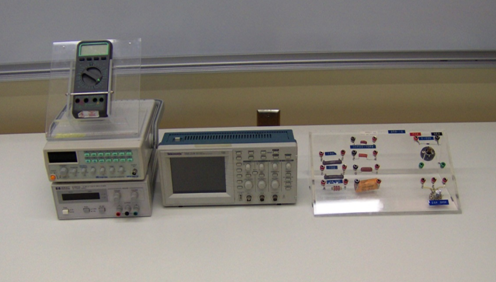
Figure 6: Equipment
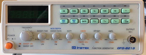
Figure 7: Function Generator
Caution:
Please, be careful in handling all of the equipment in this laboratory. The equipment is expensive and can be easily damaged if misused.
Please, be careful in handling all of the equipment in this laboratory. The equipment is expensive and can be easily damaged if misused.
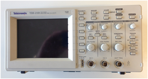
Figure 8: Oscilloscope
Procedure
Please print the worksheet for this lab. You will need this sheet to record your data.
Setting Up the Oscilloscope
1
Begin by locating the ON/OFF button on top of the oscilloscope. Press this button.
The front screen should light up. The oscilloscope will then conduct a self-test to verify the instrument is operating correctly. Wait for the confirmation that everything is OK before proceeding.
It is always a good idea to check the settings of an oscilloscope before beginning any measurements. The following is the set-up procedure to prepare the oscilloscope for the measurements in this laboratory experiment. Most of these settings are probably already preset. Just verify the settings to be sure.
The oscilloscope will always reset to the previous settings (the settings that were on the oscilloscope when it was turned off).
2
Check oscilloscope settings.
-
aPress the DISPLAY button. The settings (shown on the right edge of the screen) should be the following.
-
•Type [Vectors]
-
•Persist [Off]
-
•Format [YT]
-
•Contrast Increase (Adjustable as needed)
-
•Contrast Decrease (Adjustable as needed)
-
•NOTE: If the intensity is OK, skip this step.
-
-
-
bPress the TRIGGER MENU button. On the right side of the oscilloscope screen, there are five sections controlled by the five buttons to the right of these sections.
-
•Video [Edge]
-
•Slope [rising]
-
•Source [CH 1]
-
•Mode [Auto]
-
•Coupling [DC]
-
-
cPress the CH 1 MENU button. The four sections (in the same location as the five sections in part a above, should be set to the following.
-
•Coupling [DC]
-
•BW Limit [OFF]
-
•Volts/Div [Coarse]
-
•Probe [1x]
-
-
dPress the HORIZONTAL MENU button. The following are the sections that should be selected.
-
•[Main]
-
•Trig knob [Level]
-
-
ePress the MEASURE button. The five sections should be set to the following.
-
•Source [Type]
-
•CH 1 [Freq]
-
•CH 1 [Period]
-
•CH 1 [Pk - Pk]
-
•CH 1 [Cyc RMS]
-
-
fLocate the VOLTS/DIV knob for CH 1 and adjust it until 2.00 V is displayed on the lower left of the oscilloscope screen.
-
gThe MEASURE DISPLAY mode should remain on your screen while performing all of your measurements.
3
You are now ready to make measurements on your circuit.
Setting Up the Function Generator
1
You will now use a function generator to produce a signal on the oscilloscope. In order to prepare the generator for use, preset the control as follows.
-
aPress the POWER button (orange button on the lower left side).
-
bPress the [1k] button on the top row of green buttons.
-
cPress the [square wave] button on the second row of green buttons.
-
dAdjust the FREQUENCY control until a reading of 1.500 is displayed on the generator digital readout.
-
eThe MOD ON and MOD EXT lights should be off.
-
fRotate the AMPL knob clockwise about 1/2 turn. This should produce an output of about 10 volts.
2
The oscilloscope volts/div and sec/div settings should be:
- VOLTS/DIV 2.00 V
- SEC/DIV 250 microsec (This setting may be checked by looking at the bottom of the screen [after the symbol M].)
Measuring the Transient Behavior of a Simple RL Circuit
The objective of this experiment is to observe and measure the transient response of a series resistor-inductor RL circuit. You will also see how to use this to measure and determine the inductance in such a circuit.
1
The basic unit of inductance is henry, which is defined as the inductance necessary to produce 1 volt of EMF for a current change of 1 A/s through the device. The most commonly used units are mH (1 mH = 10−3 H).
The inductor which you will probably use will be marked with an approximate value of its inductance in mH.
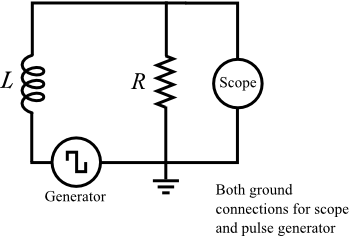
Figure 9
Finding the Value of the Inductance
2
Connect the circuit as shown in Figure 9.
3
Set the frequency of the function generator to 1 KHz (square wave), and the amplitude to maximum.
4
Set the oscilloscope as described in the Setting Up the Oscilloscope section of this experiment.
5
Connect CH 1 input of the oscilloscope across the inductor (L) in the circuit as shown.
Rotate the knobs on the oscilloscope to display the decaying voltage on the inductor such that the trace touches the top line of the screen and decays to the bottom line of the screen. The trace does not have to fill the screen (horizontally), but it does have to extend over at least 4–5 divisions in order to measure the decay constant. (See Figure 10.)
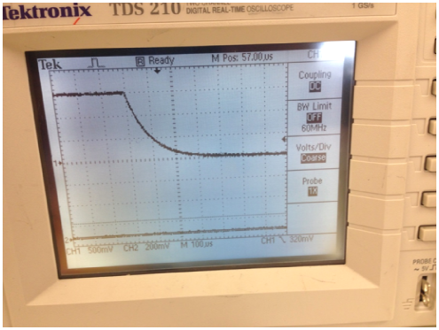
Figure 10
6
Record the voltage value of this waveform for at least 10 evenly spaced time intervals from the peak of the wave through its decay to the baseline and record these readings, in Table 1, as a time and voltage for each reading.
7
Using this data, record in Table 1 the time and the ln(Voltage).
8
Plot this as a scatter plot using Excel. Using the trendline feature in Excel, fit this curve with linear function and find the slope and intercept of this curve.
9
How are these two quantities related to the Imax, R and L of this circuit as described in Equation (7)I(t) = Ioe−t/τL.
?
10
Disconnect the resistor (R) from the circuit and measure its resistance. (Note that the internal resistance of the function generator is 50 ohms.)
11
Calculate the experimental value of the inductor (L) in the circuit using the formula τ =
,
where R is the TOTAL resistance in the circuit. Call it (experimental) L1. Do not forget the units.
| L |
| R |
12
The component value of the inductor is written on the component "bread board". Read and record this value as L2.
13
What is the percent error between the experimental value and the component value of the inductor? Which value do you consider to be more accurate? Why?
Measuring the Oscillatory Behavior of a Simple LC Circuit
1
The objective of this experiment is to observe and measure the transient response of a series inductor-capacitor, LC circuit.
2
Connect your inductor and capacitor into the circuit configuration shown in Figure 11.
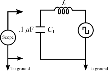
Figure 11
3
Set the frequency of the function generator to 1 KHz (square wave), and the amplitude to maximum.
4
Set the oscilloscope as described in the Setting Up the Oscilloscope section of this experiment.
5
Connect CH 1 input of the oscilloscope across the capacitor (C) in the circuit as shown.
Rotate the knobs on the oscilloscope to display the oscillating voltage on the capacitor such that the trace is centered on the screen. Since for this part of the experiment, you wish to measure the frequency of these oscillations, you will need to adjust the sweep speed to allow you to measure the time between cycles of this oscillation. Note that these oscillations gradually decay away to zero if we wait long enough. (See Figure 12.)
6
Record the voltage value for the peaks of these oscillations for at least 5 of these peaks and record these readings in Table 2. Record these readings as a time and voltage for each reading.
7
Using this data, record in Table 2 the time and the ln(Voltage).
8
Plot this as a scatter plot using Excel. Using the trendline feature in Excel, fit this curve with linear function and find the slope and intercept of this curve.
9
How are these two quantities related to the Qmax, RC of a series RC circuit? What is the value of R that you find that matches this decay time? (This decay is caused by the internal resistance of the capacitor and the inductor in the circuit.)
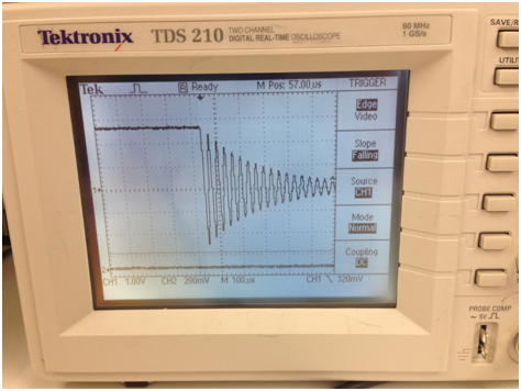
Figure 12
10
Now take this same data and measure the time intervals between successive peaks. Use this data to find the average value of the period of these oscillations.
11
How does this period compare to the period that we expect from an LC circuit according to Equation (14)ω' =
.
based on your measurement of the inductance of the inductor earlier in this lab?
 |
|
12
What is the percent error between the experimental value and the component value of the inductor? Which value do you consider to be more accurate? Why?