Faraday's Law

Introduction

This experiment examines Faraday's law of electromagnetic induction. The phenomenon involves induced voltages and currents due to changing magnetic fields. (Do not confuse this law with Faraday's laws of electrolysis, which are entirely different.) You will measure directly the voltage induced by a time-varying magnetic field and examine several effects resulting from induced EMFs. This experiment is designed to follow the Magnetic Fields experiment, since the Hall probe and the fields of coils and magnets, are examined in detail in that experiment. You should be familiar with the earlier experiment before proceeding with this one (read the Magnetic Fields write-up first in case you could not do that experiment). We know from our study of time changing magnetic field and induced EMFs that the relationship between these quantities can be expressed through the following relationship:

( 1 )

EMF_induced = −

dΦ

The negative sign in Eq. (1) gives the direction of the induced EMF. For a closed loop, one can choose either direction around the contour to be "positive." The flux is considered positive if it threads the loop in the right-hand thumb direction when the fingers point in the positive loop direction (the direction of ds). The EMF is also measured in the positive loop direction, so that for a positive EMF, E_induced tends to point along ds. With these sign conventions (as in Figure 1), Faraday's law specifies that the loop EMF will be negative if the magnetic flux increases with time, and vice versa.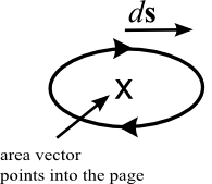

An elliptical loop has two arrows pointing clockwise placed along the loop. A third arrow above the loop points to the right and is labeled vector ds. The loop has a cross in the middle with a label indicating that the area vector points into the page.

Figure 1: Relative Directions as Defined for Faraday's Law

Another way to remember the sign of the EMF uses Lenz's Law, which states that induced currents have a direction that opposes changes in the externally applied magnetic field. Induced currents can oppose flux changes by creating a smaller flux that partially cancels the flux change. This works for conducting loops, or eddy currents in solid conductors, where the circulating induced currents are driven by Faraday's law EMFs. In addition, this idea can be used to find the EMF direction for any loop, even those that do not contain a conductor, since the direction the current would have in a conducting loop is the same as the direction of the EMF whether or not conduction is allowed. For EMFs due to changing fields, the simplest case is that of an N-turn loop of area A that remains perpendicular to a changing applied field B. If B is spatially uniform, the flux for this case will be

( 2 )

Φ = N

A · B

so that from Faraday's law, the EMF is

( 3 )

EMF_induced = −NA

If the applied field is sinusoidal, the induced EMF will also be sinusoidal. To illustrate, again consider the N-turn coil perpendicular to a uniform field with, in this case, the magnitude

( 4 )

B = B_o sin ωt.

Since

= B_oω cos ωt,

the EMF will be given by

( 5 )

EMF_induced = −NAB_oω cos ωt.

The resulting voltage has ~90° phase shift from the applied field (cosine versus sine), and is larger for higher frequencies (due to the factor of ω). This is encountered in loop-coil pickup of radio signals, and in the operation of transformers.

Objective

The objective of this experiment is for you to produce time varying magnetic fields in a region and to observe the induced EMF that is produced in such a coil. By making careful measurements of these induced fields as well as the time changing magnetic fields producing them, we will be able to verify Faraday's law.

Apparatus

Function generator
Oscilloscope
Hall probe box
Large circular coil (wound on black PVC)
Small circular coil (wound on white nylon)
Solenoid with steel core
Horseshoe magnet (with string on it)
Cylindrical magnet
Aluminum block (1 cm thick)
Plastic block (1 cm thick)
Piece of copper wire
Wooden jig

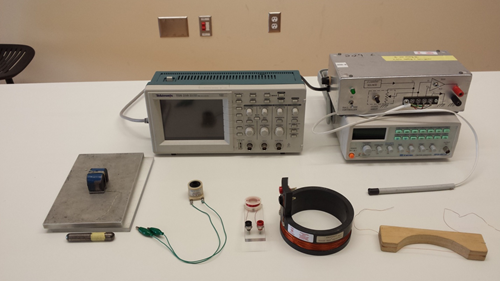
Figure 2: Equipment

Procedure

Please print the worksheet for this lab. You will need this sheet to record your data.

EMF Due to a Moving Magnet

Connect the solenoid coil to the oscilloscope CH 1 input using the BNC-to-banana cable, as in Figure 3. Set up the oscilloscope as follows:

•
trigger [AUTO]
•
sec/div.: 1 ms
•
V/div.: 0.2 V (1 x probe)
•
coupling [DC]

You will see small fluctuations in the oscilloscope trace. (If you see a large 60 Hz signal, 0.1 V or larger, one of the leads is probably not connected properly.) Small fluctuations are due to small background AC fields in the lab. Aside from these, the average voltage should be zero. Check this by switching the oscilloscope input coupling to "ground". (Is the average voltage the same as ground?) Adjust the oscilloscope vertical position so that the signal trace line is at the center of the screen. (Note: Typical background fields are about 10 mG.)

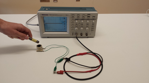
A hand holds the cylindrical magnet with one pole close to the face of the solenoid. The solenoid is attached to two alligator clips, which are connected by a BNC-to-banana cable to the oscilloscope.

Figure 3: Solenoid and Oscilloscope

With the solenoid on the lab tabletop, investigate its interaction with the cylindrical magnet (see Figure 3). Verify that you can induce a solenoid voltage (seen in the oscilloscope) by moving the magnet in its vicinity. Advance the north pole of the magnet toward the top of the solenoid. Repeat using the south pole of the magnet. Are the signs of the induced voltages the same or reversed? Describe the results.

Turn the solenoid coil over (bottom side up) and again advance the north pole of the magnet toward the coil. Are the signs of the induced voltages for this case the same or reversed from step 3?

Hold a magnet pole steadily against one end of the coil. Is there a steady voltage generated?

Verify that an EMF is generated by moving the coil toward and away from a magnet (that is on the lab table). Describe the results.

The Earth has a steady magnetic field of about 0.5 G (5 × 10^–5 T) in the laboratory. Yet, in the absence of a magnet, you should have seen no induced voltage on the coil. Why is this? Relate your answer to Faraday's law.

In moving the north pole of the magnet toward the coil, will the amount of magnetic flux in the coil be increasing or decreasing? (Think about the way that field lines emanate from a pole of the magnet.)

Are the signs of the response you recorded in steps 3 and 4 what you expect from Faraday's Law? Explain.

Explain the EMF observation you made when holding the magnet pole steadily against one end of the coil. Is there a magnetic flux in the coil in this situation?

A Moving Wire in a Magnetic Field

Example: A guitar pickup

Gently straighten about 10 cm length of the copper wire, and wrap this length around the wooden jig (you will need to wrap the ends of this wire around the two tacks on either side of the jig to get the wire taut enough for this experiment.) Make the wire segment relatively taut, and place the horseshoe magnet into the yoke with it opening facing upward with the wire between its pole tips.

Now connect the ends of this wire to the ends of the BNC-to-banana cable using the two short wires with alligator clips on each end. Connect the BNC-to banana cable to oscilloscope CH 1 input, as in Figure 4.

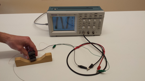
A wooden block called a jig holds two ends of a copper wire across its length. The horseshoe magnet is held so that the wire fits between the poles of the magnet. The ends of the wire protrude out from the jig. Each end connects to an alligator clip, which are connected by the BNC-to-banana cable to the oscilloscope.

Figure 4: Wire Segment and Oscilloscope

Set the oscilloscope to:

•
trigger [AUTO]
•
horizontal sec/div.: 20 ms
•
vertical V/div.: 5 mV (1 x probe)
•
coupling [DC]

Adjust the oscilloscope display so that the line trace is located near the center of the screen.

Caution:
There are exposed connector tips at the ends of the test lead; watch that these do not touch each other and short out your observation.

You now have a magnetic pickup as is found in an electric guitar (the wire being the guitar string). Pluck the wire, and observe the result in the oscilloscope. What is the maximum voltage amplitude you can obtain in this way?

Try shaking the wire slowly back and forth; is the amplitude the same?

If you wanted to improve your pickup circuit so as to obtain larger signals, which changes might help: a larger magnetic field, a thicker wire, a smaller wire resistance? Why?

Measurements with Time-Dependent Fields

Locate the Hall probe box on the lab table. Set the gain on the box to xl00. Turn the filter off. Connect the Hall probe output to the oscilloscope CH1 input. The oscilloscope settings should be:

trigger [AUTO]
sec/div.: 2.5 ms
V/div.: 2 mV (1 x probe)
coupling [AC]

Connect the large circular coil to the function generator output. Set the frequency to 100 Hz (sine wave), and the output to its maximum value. Place the coil flat on the bench top.

Hold the Hall probe at the center of the large coil. Observe that the oscilloscope indicates a voltage proportional to the time-dependent field, for each of the three functions (sinusoidal, triangle, square). (The noise is intrinsic to the Hall probe; you should aim to find the center of the trace, since the fluctuations are equally positive and negative.)

In the procedures to follow, the probe and the large circular coil must be held in line with each other to obtain accurate readings. As you recall, field lines for a circular coil, observed on the axis, lie parallel to the axis (up and down in this case).

Set aside the large coil and locate the small circular coil. Connect it to the input of the oscilloscope (in place of the Hall probe box output). Holding the small coil at the center of the large coil, observe the waveforms on the oscilloscope for each of the three functions of the function generator (Figure 5). Sketch the waveform shapes for each case using the screen template supplied and the Paint program. Are these equivalent to the derivatives of the magnetic field waveforms?

Note: You may need to adjust the trigger level in order to stabilize the waveform on the oscilloscope screen. The trigger level should be around the middle of the amplitude for the waveform for best rest results.

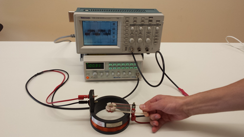
Two coils are at the center of the image. The large coil sits atop the table and is connected by cable to the function generator. The small coil is held above the large coil and is connected by cable to the oscilloscope.

Figure 5: Coils and Oscilloscope

Connect the Hall probe box to the oscilloscope once more. Hold the Hall probe steadily at the center of the coil. Set the function generator for a triangle wave. Measure the voltage rise (ΔV) and the elapsed time (Δt) for part of the wave from the Hall probe box.

From this, calculate the slope

ΔV

Δt

Use the calibration on the Hall probe box to convert this to the rate of change of magnetic field,

Having done this, connect the small coil to the oscilloscope again, place the coil at the center of the large coil, and measure the amplitude of the induced EMF, in volts, directly from the oscilloscope. (The amplitude is half the peak-to-peak value.)

Repeat this last procedure: Connect the Hall probe box to the oscilloscope, change the function generator to a sine wave, and measure the amplitude of the wave (half the peak-to-peak voltage). The frequency should still be 100 Hz, and the Hall probe should be in the center of the coil. Convert your measured amplitude from the oscilloscope to a magnetic field in T using the calibration on the Hall probe box. Now connect the small coil to the oscilloscope and hold the pickup coil in the center of the large coil. Record the amplitude of the sinusoidal EMF observed in the oscilloscope.

The small circular coil contains 50 turns. Take the average diameter to be 2.05 cm. With this information, and the rate of field change

you measured in step 6, calculate the steady EMF predicted from Faraday's law. Does the calculated result agree with your measured EMF?

With a sinusoidal magnetic field, Faraday's law predicts an

EMF_induced = −NABω cos ωt,

as described above. With the amplitude of the sinusoidal field that you have just measured, calculate the predicted EMF amplitude. You must first convert Hz to radian/s. Does this agree with the value you observed?

Magnet Brake and Eddy Currents

Magnet Braking

Suspend the horseshoe magnet by a string over the lab table. Remove the magnet's keeper bar, if it is not already removed.

Spin the magnet on its axis on the end of the string. With some care this can be done so that the magnet rotates in place, with little wobbling. Note that the magnet will spin for some time without stopping, alternately winding and unwinding the string. Watch this behavior of the spinning magnet for a few cycles.

Now, bring the aluminum block close to poles of the spinning magnet without touching it by sliding it under the spinning magnet. Is there an effect? Record your observations.

Repeat with the plastic block. Is there any difference?

Eddy Current Propulsion

Hold the suspended magnet at rest a centimeter or two above the aluminum block that is resting on the table top.

Being careful not to touch the magnet, have one of your lab partners gently pull the aluminum away horizontally. Observe and record the effect on the magnet.

What happens when you reverse the direction of the movement of the aluminum block?

Now try this with the plastic block and observe that the effect cannot be due to air currents.

The actual shape of the eddy currents in this part is quite complicated. However, can you make a general statement about forces and the relative motion of magnets and conductors?