
Motion in One Dimension
Introduction
The object of this lab is to help you gain understanding of motion in one dimension. We shall study the motion of a low friction air cart as it moves down a linear air cushioned track inclined at an angle θ. The motion along the track is one-dimensional and we shall choose the direction along the track to be the x-axis. The acceleration of the cart along the incline should be approximately constant and equal to g sin θ, where g = 9.81 m/s2 is the acceleration due to gravity. If we start the cart from rest at t = 0, and x = 0, then at time t, the speed vx and the position x of the cart are given by:( 1 )
vx = at, and x =
at2
| 1 |
| 2 |
vx = at, and x =
at2
, we obtain the following relationship between vx and x.
| 1 |
| 2 |
( 2 )
vx2 = 2ax
Procedure
In the first part of this experiment, we shall verify Eq. (1)vx = at, and x =
at2
by measuring the position of the cart as a function of time. In the second part of the experiment, we shall verify Eq. (2) | 1 |
| 2 |
vx2 = 2ax
by measuring the speed vx of the cart as a function of the position x.
Change of Position with Time
The experiment will use a very low friction air cart that runs on a cushion of air. This equipment is expensive, so please treat it well. You will use a stopwatch to measure the time it takes for the cart to reach a predetermined position. Note that the stopwatch you will be using is precise to 0.01 seconds, but your reflexes probably are not. Thus the measurements made here will not be highly accurate, and a careful error analysis will be needed to justify any conclusion that you make.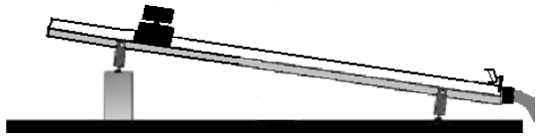
Figure 1
Note: The air track should be set up with an incline angle of 2 to 4 degrees.
-
1Use a digital level to make several measurements of the angle θ that the track makes with the horizontal. Do so by placing the digital level on an aluminum "V" block that is designed to rest on top of the air track. Note that the digital level measures the angle from true horizontal, so it is not necessary to "zero" the level before taking a measurement.
-
2Turn on the air supply. The cart should move freely along the track.
-
3Practice timing the cart as it moves down the inclined air track a few times to acquaint yourself with the operation of the stopwatch. (Note that you can use either the hand held one or the one incorporated into the base of the photogate/timer).
-
4Let the cart go from rest from some pre-determined position that you will designate asx = 0.Using the stopwatch, measure the time it takes the cart to travel 0.4, 0.6, 0.8, 1.0 and 1.2 meters. (You must start the cart from rest at 0 meters for each measurement). Repeat each trial several times, and enter the results of your measurements into a data sheet. You should repeat a trial if you think it went badly, for instance you hit the stopwatch button too soon or late. If you repeat a trial, do record the results of the bad trial and justify your omission of that data. To reduce reaction time errors, the same person who is using the stopwatch should release the cart.
-
5Observe that the velocity of the cart will increase with time. Can you tell that the rate at which the cart's velocity increases is constant?
Velocity at Different Positions
One way to find the cart's velocity at position x is to simply time how long, Δt, the cart takes to go a small known distance, Δx, when it is passing the position x and use the equationvx = Δx/Δt.
You are still finding an average velocity by this method, but it is a good approximation of the cart's instantaneous velocity at x when Δt is small. The small time interval, Δt, can be measured precisely by using the lab counter/timer and the photogate.
-
1Measure the length, Δx, of the flag on the cart. Carefully position the photogate over the track so that the velocity of the cart will be measured after it has traveled a fixed distance x from rest. Show on your data sheet (words and/or sketch) how you line up the cart with the zero mark, and show the placement of the photogate relative to the position x. (Be sure you are clear: the timer reports the time of passage of the cart, not the cart's velocity.)
-
2To make the measurement, simply release the cart and allow it to pass through the photogate. Record the time, Δt. Repeat the measurement several times at each of the positions x = 0.4, 0.6, 0.8, 1.0, 1.2 meters. Record your measurements on your data sheet.
Be sure that you and your TA each initial your worksheet.
Analysis
Position as a Function of Time
To check if the motion of the cart is described by Eq. (1)vx = at, and x =
at2
, you will make a plot of t2 vs. x (i.e. t2 on the y-axis and x on the x-axis). If indeed the acceleration is constant, the plot should produce a line described by:
| 1 |
| 2 |
( 3 )
t2 =
| 2x |
| a |
-
1Calculate a = g sin θ and its uncertainty. The uncertainty can be calculated using the upper-lower bound method with the range of angle measurements (see Error Analysis chapter).
-
2Prepare a table (Table I) to record the data you need for this plot.
-
3Plott2vs. x including error bars fort2.Perform a least-squares linear fit to your data and use Eq. (3)t2 =to determine the acceleration a and its uncertainty from the fitting parameters.
2x a
Velocity as a Function of Position
vx2 = 2ax
To examine the validity of Eq. (2)vx2 = 2ax
, we will make a plot of vx2 vs. x.
-
1Calculate the velocity of the cart at each position x, using vx = Δx/Δt and the data for Δt from the data sheet. For each position x, find the average of vx2 over the number of trials you have made and calculate its standard error. Present the results of your analysis in a table (Table II). Your table should contain columns for:
-
•x
-
•avg. (vx2)
-
•the uncertainty of vx2
-
-
2Make a plot of vx2 vs. x including error bars for vx2.
-
3Make a least-squares linear fit to examine Eq. (2)vx2 = 2ax. Determine the acceleration a and its uncertainty from the fitting parameters.
Discussion
Summarize your results, i.e. your two values for the acceleration together with their uncertainty. Is the motion of the cart consistent with the equations of motion for constant acceleration Eq. (1)vx = at, and x =
at2
and Eq. (2)| 1 |
| 2 |
vx2 = 2ax
? Why or why not? Does the value of the acceleration found from the two different procedures agree with g sin θ? Explain. Which of the values is more precise? Which is more accurate? How can you tell? What are the most significant systematic errors in this experiment and how do they affect your results?