
Interference and Diffraction of Light
"No one has ever been able to define the difference between interference and diffraction satisfactorily. It is just a question of usage, and there is no specific, important physical difference between them. The best we can do, roughly speaking, is to say that when there are only a few sources, say two, interfering, then the result is usually called interference, but if there is a large number of them, it seems that the word diffraction is more often used."—Richard Feynman's Lectures on Physics, Vol. 1
Purpose
-
•To observe the behavior of light passing through various configurations of slits.
-
•To investigate how the width of a slit and the wavelength of the light passing through it determine the diffraction of light.
-
•To determine the wavelength of laser light from the diffraction pattern produced when it passes through a single slit.
-
•To determine the wavelength of laser light from the interference pattern produced when it passes through a pair of slits.
-
•To measure the width of a narrow slit from the diffraction pattern produced when laser light passes through it.
-
•To investigate the role played by single slit diffraction in the variation in intensity of a double slit interference pattern.
Equipment
- Virtual Diffraction simulation
- Pencil
Explore the Apparatus
Open the Virtual Diffraction simulation on the website.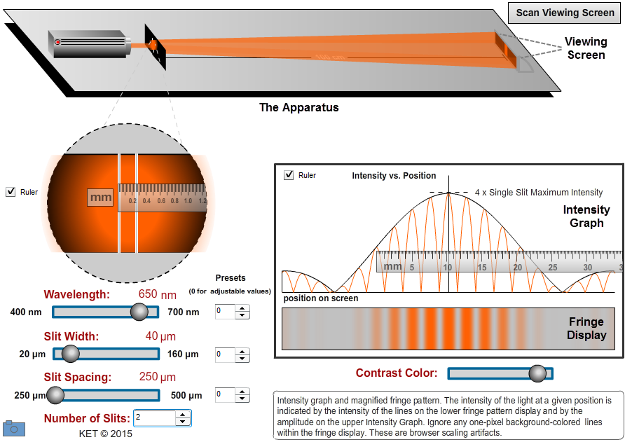
Figure 1: Interference and Diffraction Apparatus
-
•the height of the Intensity Graph, which is a plot of the intensity of the light vs. position on the Viewing Screen.
-
•the brightness of the bars of light, called fringes, on the small Viewing Screen on the apparatus, and in the enlarged replica of this interference pattern in the Fringe Display below the Intensity Graph.
-
•The wavelength can be adjusted throughout the typical visible (human) range of 400 nm to 700 nm.
-
•The width of the slits can be adjusted from 20 µm to 160 µm.
-
•The slit spacing, the distance between the centers of adjacent slits, can be adjusted from 250 µm to 500 µm.
-
•The number of slits can be varied from 1 to 5.
The first three parameters also have several preset unknown values. In your WebAssign assignment, you'll be given a random "unknown number"—the number which you'll use to select your unknowns. So if you are told to use your assigned unknown wavelength and your unknown number is 2, you'll just select "2" with the wavelength stepper.
-
•slit width and slit spacing. (Zooming in is recommended here.)
-
•position of a minimum or maximum point relative to the central maximum on the Intensity Graph.
1
Drag the wavelength slider all the way to the left. We'll call this color violet. What's its wavelength?
2
Drag the wavelength slider all the way to the right. We'll call this color red. What's its wavelength?
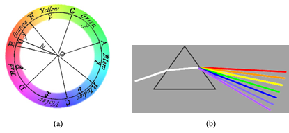
Figure 2: (a) From Newton's Optiks; (b) From Pink Floyd's Optiks
For humans there's a range of wavelengths that could be called red, a range called orange, etc. We, like Newton, find that as we move through the colors from red to violet, we come upon about six or seven with widely agreed upon names and hues. His representation of the colors as a continuum doesn't correspond to any real behavior. And indigo might be a stretch for most of us.
3
It's useful in our work to know about the order of these colors in the spectrum and how they relate to wavelengths. So, let's get to know them. Select a wavelength in the range of each color in the sequence ROYGBIV. There are no exact answers. Just try again if your estimate is rejected and blame it on your monitor.
-
aRed
-
bOrange
-
cYellow (very narrow)
-
dGreen
-
eBlue
-
fIndigo no way
-
gViolet (very narrow)
4
Set the laser color to a red, the number of slits to one, and the slit width to 40 µm. Scan. (This means to click the Scan Viewing Screen button.) You should see a nice red "fringe" that takes up about half the width of the Fringe Display. Two other very dim fringes appear just at the edge of the Fringe Display. Adjust the background contrast as needed. Zoom in three times on the Viewing Screen on the apparatus. The Fringe Display just shows the central part of this full, but tiny, display. Zoom back out to 100%.
5
Slowly adjust the wavelength from red to violet. Scan.
As the wavelength decreases, the width of the central, bright fringe
. (increases or decreases)
6
Reset the color to red. Scan. The slit width should be set to 40 µm. Slowly increase the slit width to its maximum value. Scan. What three significant changes do you observe as you increase the slit width? One involves the Intensity Graph.
7
Reset the slit width to 40 µm. Scan.
Change the number of slits to two. Scan. Describe the changes in the Fringe Display and the Intensity Graph. Also comment on what stays the same.
8
Feel free to change the number of slits up to 5 and Scan if you like spiky things.
Theory
A. Diffraction and Interference
While you're waiting for your opponent to arrive at the tennis court, you can warm up by hitting the ball against a wall. You can count on the ball to behave in a predictable manner. If you have good aim, the ball is always going to bounce back. If you hit it past either side you know right where to go to pick it up. So unless you hit the ball over the wall the area behind the wall is a tennis ball shadow. If you do hit the ball over the wall and some kind person on the other side throws it back over the wall to you, you don't have to climb the wall or walk to the edge of the wall to shout your thanks. Not only can you just shout toward the wall, you can shout in almost any direction and still be heard. Clearly sound doesn't behave like a tennis ball. There is no sound shadow behind the wall. There are actually two phenomena involved in this "hearing around corners" phenomenon. When the sound arrives at an edge of the wall, it bends around the wall. This "bending" of waves when they reach an opening or an edge is called diffraction. So how does the sound get behind the wall when you don't even shout in the direction of the wall? It diffracts when it exits your mouth. Differently shaped speakers for different situations and cheerleading megaphones suggest that there are ways of modifying the amount and direction of diffraction. There's another factor involved in talking to someone behind the wall. If you or your listener were to move around a bit you'd find that the sound heard would be clearer and louder at some points and more garbled at others. This is because all this sound wrapping around and over the wall is recombining at your listener's ears to reproduce the pattern of compression and decompression of the air that you originally produced.
Sound coming by different paths will be out of sync to different degrees, so what's heard is a mash up of different parts of "Thank you very much for returning the ball." Something like:
|
|
 |
"HUH? All I got was a bunch of noise ending with bbball." |
B. Interference
Let's look at the interference of a pair of waves on the surface of a tank of water. Figure 3 is a snapshot of a red marble jiggling up and down when partially submerged in a tank of water. A continuous circular surface wave is produced. The small bit of Styrofoam jiggles up and down with a slight delay due to the travel time of the wave.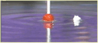
Figure 3: Water Waves
| r |
| 2 |
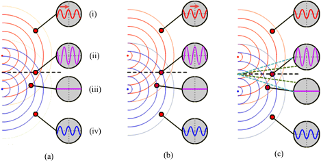
Figure 4: Interference of Two Overlapping Circular Waves: (a) In Phase—Trough
(b) In Phase—Crest (c) Nodal and Antinodal Lines
(b) In Phase—Crest (c) Nodal and Antinodal Lines
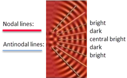
Figure 5: Nodal and Antinodal Lines in Water; Bright and Dark Fringes on a Screen
Equations for the location of nodal (dark) and antinodal (bright) fringes
We've found that points of constructive or destructive interference are due to the difference in distance, the path difference, Δr, between the sources and positions on a screen. (This assumes that the sources are in phase, which they'll always be with this apparatus.) Specifically, if light travels λ, 2λ, 3λ, etc., farther from one source than from another, then constructive interference will occur. Similarly, destructive interference will occur if the path difference is 0.5λ, 1.5λ, 2.5λ, etc. In Figure 6, light sources S1 and S2 produce identical waves in phase. Since r1 and r2 are equal distances, all waves will arrive at point P in phase. Crests will arrive together, as will troughs. So point P will be a bright fringe. Due to the symmetry of the arrangement, we would call it the central bright fringe. This corresponds to point (ii) in Figures (4a–c).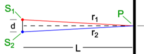
Figure 6: Central Bright Fringe
r2 − r1 = λ/2.
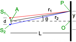
Figure 7: First Order Bright Fringe
L >> d,
the mathematics is much simpler than what we see in Figure 7. We'll just deal with this case, which was developed by Joseph Fraunhofer. (See the "Cosmos: A Spacetime Odyssey" "Hiding in the Light" episode to see how we almost lost young Joseph. He was fortunate to have a house fall on top of him.)
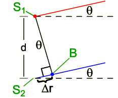
Figure 8: First Order Bright Fringe, where L >> d
Δr = λ.
For the next bright fringe, at a larger angle, θ, Δr = 2λ,
and so on. Similarly, for dark fringes we'd have Δr =
λ,
λ,
and so on.
For two sources, created in phase, at a distance L from a screen:
We use ±m values to distinguish fringes on either side of the central maximum.
Using right triangle ΔS1S2B, in Figure 8, and noting that d is the distance between S1 and S2, we can say
Substituting each expression for Δr into equation 3, we can solve to find
One practical problem with equations 4 and 5 is that it's difficult to precisely measure these very small angles. The geometry of Figure 7 suggests an alternative. Again assuming that | 1 |
| 2 |
| 3 |
| 2 |
L >> d,
we can use the large triangle ΔAOP to produce the equation
In addition, we know that for small angles tan θ ≈ sin θ.
So we can solve equation 6 for tan θ and substitute the result for the sin θ term in equation 4 to get
Procedure
Please print the worksheet for this lab. You will need this sheet to record your data.
I. Double Slit Interference–Measuring an Unknown Wavelength
So how might we arrange for two sources of light to come together in phase, or out of phase, on a screen? You've probably read about a modified version of Thomas Young's famous experiment in 1801 that involved light passing through a single slit, then through a pair of closely spaced slits, and then being viewed on a screen in a darkened room. Using light from this single source to illuminate both slits insured that the light coming from the two slits was in phase. A more convenient method unavailable to Thomas Young by about 150 years is to use laser light. Due to its method of production, laser light is always in phase. In Figure 9, laser light diffracts separately through each slit, providing us two in-phase sources of light to illuminate our screen. We'll now set up our virtual apparatus in this two-slit mode, and use equations 1–7 to determine the wavelength of our monochromatic laser light.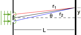
Figure 9: Monochromatic Laser Light Through Two Slits
ym =
where m = 0, ±1, ±2, . . . for bright fringes. (double slit)
to calculate the wavelength of a shade of light in the green-yellow region and then repeat the process with your unknown wavelength. In each step below, you'll want to record your settings, measurements, and calculated values in Table 1 in your WebAssign assignment.
| mLλ |
| d |
Be careful with units. The table conveniently uses four different units of length to correspond to the apparatus display units and ruler units. You'll inconveniently need to convert each of these units to meters when you do calculations. It could be worse. You could have a house fall on you.
1
Set the number of slits to two, and the slit spacing, d, to 250 µm. (µ, micro = 10–6, n, nano = 10−9).
2
Set the slit width, w, to 40 µm.
3
Turn on the laser. Adjust the wavelength slider to 540 nm. Notice how the apparatus—laser, slit, and screen—matches our assumptions about d, L, θ, etc. Rays traveling from the two slits to a given point on the screen are very nearly parallel. In the following images, a red-orange wavelength will be used as an example. Your green-yellow wave y-values will be smaller than those shown. (The green doesn't print out very well on paper.)
4
Scan to record and display the intensity data. You'll see a set of yellow-green fringes of varying brightness. The bright fringes are maxima, and the minima are in between. The specific location of a maximum is at its brightest point. As you can see, this is hard to determine from the thick fringes.
The Intensity Graph takes care of that problem. The scanning photodetector measures the intensity of the light reaching the Viewing Screen at each horizontal position on the screen. This intensity data is plotted so that the height of the curve corresponds to the brightness of the light measured by the photodetector at a given point. This curve more precisely shows the variation in brightness of the light.
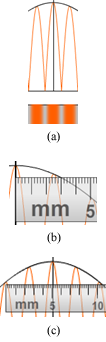
Figure 10: (a) Maxima and Minima (b) Position, ym, of a Maximum (c) –y2 to +y2
We'll use the distance from the center line out to a peak as a measure of the position of the maximum. (Use the checkbox to turn on the mm ruler.) In Figure (10b), that would be about 2.5 mm for the first maximum and about 5.1 to the second maximum. Be sure to note that the smallest increments on the ruler are 0.2 mm apart. The position of a maximum is represented by ym, where m is the order of the maximum. The maximum at 2.5 mm in Figure 10 is y1 since it's the first one-to-one side of the central maximum. There's another first order maximum equidistant at –y1 on the left.
To improve our accuracy we'll take advantage of the equal spacing of the maxima. Figure (10c) shows the m = 1 and 2 peak on either side of the central maximum. The ruler shown is aligned to measure the distance between –y2 and +y2. By zooming in a couple of times, you should be able to measure this distance to 0.1 mm. Since this is the span of four maxima, half of that distance would be y2. If that total distance is 10.2 mm, then y2 would be 5.1 mm.
Note:
Any time you make a change in the parameters—wavelength, slit width, etc.—you'll need to Scan to reset the Intensity Graph.
Any time you make a change in the parameters—wavelength, slit width, etc.—you'll need to Scan to reset the Intensity Graph.
5
Measure the distance between –y3 on the left and +y3 on the right.
6
Calculate y3 by dividing the –y3 to +y3 distance by 2.
7
Calculate θ3, the angle for the third maximum, using equation 6y = L tan θ.
. For your results to be valid, θ must be less than a few degrees. You should get a very tiny angle. (Be careful to use meters for all distances in your calculations!)
8
Use equation 7ym =
where m = 0, ±1, ±2, . . . for bright fringes. (double slit)
to determine the experimental value of the wavelength of your laser light.
| mLλ |
| d |
9
Compare your experimental value to the theoretical value by calculating the percentage error.
10
Show your calculations of θ3, λ, and your percentage error.
11
Adjust the laser to your assigned wavelength by setting the numeric stepper to your unknown number.
12
Collect all the data and calculate all the values you need to fill in the trial 2 row of Table 1.
13
Show your calculations of θ3 and your wavelength.
Figure 11: The Geometry of Interference Patterns
14
In Figure 12, the first maximum you just produced is shown as y-original, y0. But the slits have been adjusted to be twice as far apart. The first maximum will now be at a new point which you need to find using the diagram. What effect would doubling the slit spacing have on the location of this first maximum? Add the missing lines from Figure 11 to this figure taking into account the new positions of the centers of the slits. It takes a bit of trial and error. Fortunately you're using a pencil.
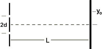
Figure 12: The Effect of Slit Spacing on the Location of Maxima
15
You should now be able to make an estimate of what would happen to your trial 2 data if you doubled the slit spacing.
-
aWhat was your value that you recorded for the distance "–y3 to +y3" from trial 2?
-
bWhat do you predict will be the value for "–y3 to +y3" if you double the slit spacing?
16
Now test your prediction with your assigned wavelength. Double the slit spacing from 250 to 500 µm. Scan. Measure y3 with the new spacing. Enter your data as trial 3 in Table 1.
Let's summarize some of the basic ideas that you've learned so far. For light passing through a pair of narrow slits, how is the spacing of the fringes affected by
-
athe spacing of the slits?
-
bthe wavelength of the light?
-
cthe distance from the slits to the screen (you weren't able to test this with the apparatus, but geometry helps)?
II. Single Slit Diffraction
When we looked at the interference of a pair of circular water waves in Part B of the theory, we found alternating maxima and minima just as we've found with a pair of slits. But there's something else going on that we haven't addressed. The fringe brightness drops off with increasing y-values. But then it increases at larger y-values! There's nothing about our water wave model that would suggest this behavior. Back to the lab!
Figure 13: Brightness vs. y
1
Reset your apparatus to the arrangement we used in trial 1 in Part I. That is, two slits, λ = 540 nm,
slit width, w = 40 µm, slit spacing, d = 250 μm.
Scan.
2
In Figure 14 draw a simple sketch of what you observe on the Intensity Graph and Fringe Display.
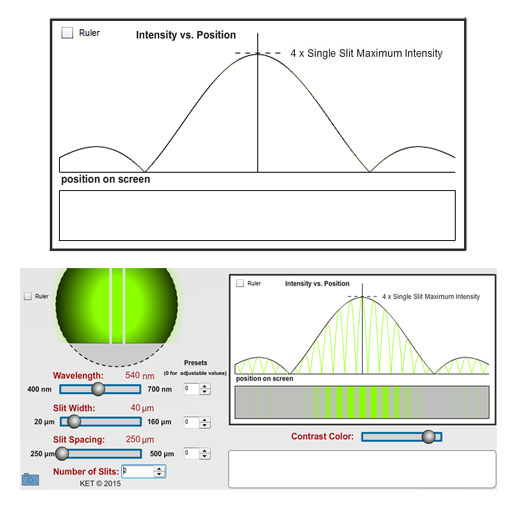
Figure 14: Double Slit Intensity and Fringe Pattern
3
Take a Screenshot of the bottom portion of the lab screen—the part below the apparatus. Upload it as "interference_doubleslits.png".
4
Decrease the number of slits to one. Scan. What a difference a slit makes! You commented on this in your initial exploration. There are some obvious as well as some subtle things that occur when you switch from two slits to one. The multiple individual fringes are replaced by a wide central fringe and two very dim fringes on either end. Also, the varying brightness (intensity) of the original, double slit fringes is reflected in the varying brightness of the three single slit fringes at corresponding positions. If you didn't notice that, switch back and forth between one and two slits. Be sure to Scan after each switch. Also, the shape of the intensity curve of the single slit fringe pattern is identical to the shape of what we call the envelope of the double slit intensity curve.
To be clear about what we're observing, the intensity of the double slit curve is very spiky. But if you draw a smooth curve connecting the maxima of all the spikes, you get what's called the envelope of the intensity graph. That envelope looks just like the intensity graph of a single slit. (We'll address the intensity scale differences later.)
Why is this happening? Perhaps the variation in brightness with position on the Fringe Display is some sort of individual slit behavior and the number of fringes is a multi-slit behavior. To understand why this occurs we need to observe the behavior of light passing through just one slit.
5
In Figure 15 draw a simple sketch of what you observe on the Intensity Graph and Fringe Display for the one-slit case.
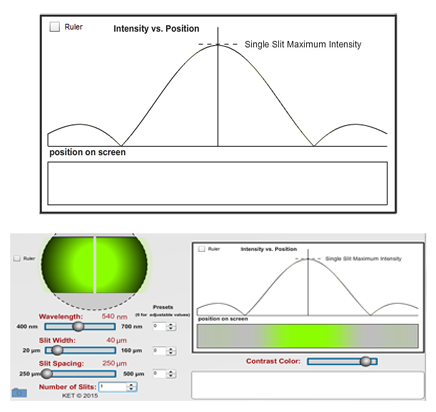
Figure 15: Single Slit Intensity and Fringe Pattern
6
Take a Screenshot of the bottom portion of the lab screen—the part below the apparatus. Upload it as "interference_singleslit.png".
Slit Diffraction/Interference
In Figure 4, we saw the interference pattern produced by of a pair of point sources, which produced circular waves in all directions. We then created a similar effect with light by using a pair of slits. But we also found an unexpected feature—the variation in brightness—something that our water wave model would not have predicted. The difference is due to the finite (as opposed to extremely narrow) size of our slits. Our slits are not really point sources. To understand why this is important, we first need to consider how waves actually travel through our slits. Christian Huygens developed a principle that explains how a wave front propagates, that is, how a wave front at one instant can produce a new wave front at a new position a short time later. He suggested that each point along a wave front acts as the source of tiny circular wavelets that move forward at the wave's speed. The wave front a moment later is the tangent to all these individual wavelets. In Figure (16a), we see a section of a long, straight wave traveling toward a narrow slit. The second wave from the left is shown producing three Huygens wavelets which result in a new straight wave. A wave produced three periods earlier is nearing the slit. In Figure (16b), just a tiny part of the wave has passed through the slit, leaving just the circular wave from that point-like section of the original wave to continue on. This is the behavior of waves passing through a very narrow slit—the waves act almost as if they're all coming from the same point, much like our water waves! As mentioned before, this bending into what would be expected to be shadow is called diffraction. Figures (16a) and (16b) demonstrate a case of strongly diffracted waves.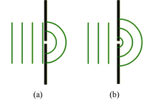
Figure 16: Diffraction by a Narrow Slit
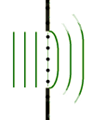
Figure 17: Diffraction by a Wider Slit
7
Let's watch this happen with our apparatus, still with one slit. All of our work is being done with slit widths of at least 40 µm. Use that width and λ = 540 nm. Look at the Viewing Screen on the apparatus. You should see a very tiny bright fringe at the center of the screen. Zoom in several times. You should see the central bright fringe, then the faint m = ±1 fringes and then some still fainter m = ± 2 fringes.
The light passing through a 40 µm wide slit has expanded so that the central maximum is about 27 mm wide. The angle of this wedge of light is only about 1.6°. Now zoom back out.
8
Gradually slide the slit width slider to the left to 20 µm while watching the Fringe Display. Scan.
The central bright fringe fills the whole Intensity Graph. This is approaching, but still far away from what Figures (16a) and (16b) are illustrating—point source behavior. It's also closer to what the individual water waves did in Figures (4a) and (4b). Their amplitude seemed to be unrelated to θ. You should be able to picture the result of further reduction in slit width.
9
There's another factor that influences the amount of diffraction. Return the slit width to 40 µm. Drag the wavelength slider back and forth and notice the change in width of the diffraction pattern. Obviously the wavelength plays a key role in diffraction, too.
10
When light passes through a narrow slit, the amount of diffraction
with wavelength and
with the width of the slit. (increases or decreases) So diffraction is proportional to λ/w.
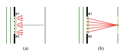
Figure 18: (a) Light Produced by Wavelets (b) Central Bright Fringe
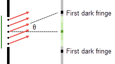
Figure 19: First Dark Fringe
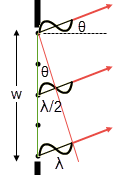
Figure 20: Production of First Dark Fringe
| 1 |
| 2 |
11
For the first dark fringe on a screen and slit width w, as the wavelength, λ, increases, the angle θ
.
12
For the first dark fringe on a screen and wavelength λ, as the slit width, w, increases, the angle θ
.
sin θ = λ/w
and
Equation 8 was produced by dividing the slit into two sections so that each wavelet in the top half had a matching wavelet in the bottom half that would destructively interfere with it. If we divide the slit into four sections, the top two will destructively interfere and the bottom two will destructively interfere. This will work with any even number of divisions.
For example, for the second dark fringe, the wave from point 5 must travel λ farther than the wave from point 3 and point 3 must travel λ farther than point 1. Thus, equation 8 becomes w sin θ = 2λ.
So sin θ will be twice what it was for the first dark fringe. In general, for all dark fringes produced by a single slit,
Again, for small angles we can also use the small angle approximation, 
sin θ = tan θ = yn/L
to produce
Example:
Set the wavelength to 550 nm and the slit width to 100 µm. Scan. We'll solve for the slit width, w, for our example. You should see one central peak and three full shorter peaks on either side. But we're interested in the dark fringes, not the bright ones. (You can see how they're easier to measure.) We have four dark fringes on each side. So m = 4 and the distance between these dark fringes, referred to in the table as
which is the 100 µm we expected.
This would be a handy technique for anyone needing to measure the width of small openings. We live in a nano-world.
Set the wavelength to 550 nm and the slit width to 100 µm. Scan. We'll solve for the slit width, w, for our example. You should see one central peak and three full shorter peaks on either side. But we're interested in the dark fringes, not the bright ones. (You can see how they're easier to measure.) We have four dark fringes on each side. So m = 4 and the distance between these dark fringes, referred to in the table as
y−4
to y+4, is about 43.9 mm. So y4 = (0.0439 m)/2. Solving equation 10 for w and entering our data gives a value for w of about
w =
=
= 100\,µm
| mLλ |
| ym |
| 4 × 1 m × 550 nm |
| (0.0439 m)/2 |
13
You've found your assigned unknown wavelength previously using the double slit equations. Let's find that value again with our single slit equation. Use a slit width of 40 µm. Take whatever data you need and enter it and your results as trial 1 in Table 2.
14
Calculate the percent difference between the values you determined for your unknown wavelength with the single slit and the double slit calculations.
15
Show your calculations for the experimental value of your wavelength.
ym =
where m = 1, 2, 3, . . . for dark fringes. (single slit)
to measure the width of one of the six slits of unknown width.
| mLλ |
| w |
16
Use the numeric steppers beside the wavelength and the slit width sliders to select your unknown number for each of these. Leave the slit spacing at 250 µm and set the number of slits to one.
17
Enter your just-determined experimental value of your unknown wavelength under the λ (nm) column.
18
Take your y-data to determine your slit width.
19
Show your calculations of the unknown slit width in trial 2. You'll need to show your calculation of ym and w.
If you run into trouble, try some known values to test your math.
III. Two Slit Interference with Single Slit Diffraction
We've mostly been dealing with slits that are less point-like than our water waves, and as a result, they each produce the diffraction patterns we've seen with single slits. We'll now examine their role in producing the interference patterns we've been observing with double slits.1
Set up your apparatus with wavelength #2 and slit width #1. Leave the slit spacing d = 250 µm.
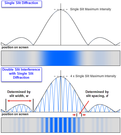
Figure 21: Double Slit Interference with Single Slit Diffraction
2
Increasing the slit spacing, d, will
the number of bright fringes in Figure 21. (increase, decrease, not affect)
3
It will
the widths of the peaks of the envelope. (increase, decrease, not affect)
4
Replacing the blue light with
will reduce the distance between the two first order (m = 1) dark fringes of the double slit pattern. (violet, red)
5
Thus we can say the spacing of the bright fringes is
proportional to wavelength. (directly, inversely)
6
the widths of the slits will reduce the distance between the two first order (m = 1) dark fringes of the double slit pattern. (Increasing, Decreasing)
7
Thus we can say that the spacing of the dark fringes is
proportional to slit width. (directly, inversely)
Intensity of Single and Multiple Slits
There is one final observation that we've been skirting up to this point—the intensity of the light for single and multiple slits.8
Reset your apparatus to two slits, λ = 540 nm, slit width w = 40 µm, slit spacing d = 250 µm. Scan. (As before we'll use a better color for printing in our figures.)
We want to keep an eye on one arbitrary location on the screen. Let's use the y3 fringe on the left. Notice the brightness of that fringe. Also notice the corresponding height of the Intensity Graph at that location.
Figure 22: y3 Intensity
9
Switch back and forth between one and two slits. Don't Scan. Just compare the brightness of the light and height of the graph at the y3 point for each case. They seem to be exactly the same. Is that correct? Let's look at the dark fringes on either side of y3 first.
Set the number of slits to 2. The dark bands on either side of y3 were caused by destructive interference of light coming from each of the two slits as given by equation 5 |
| 1 |
| 2 |
 |
10
What about the y3 maximum? If one slit provides light of a certain brightness at that point, what brightness should we expect if light from a pair of slits interferes constructively at that point? Twice as much?
11
Click the "Number of Slits" stepper to change the number to 1. Notice the label to the right of the peak of the graph. This establishes the intensity scale for the graph. If you move your pointer across the graph, this label will disappear. Moving your pointer over "Intensity vs. Position" will always bring it back.
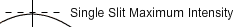
Figure 23: Single Slit Scale
12
Now for two slits. If we were right about the intensity being twice as much, we'd expect the graph to be twice as high. Right? But we don't have room. So we'll adjust the scale instead. Change to two slits and note the scaling label. What gives?
Actually, all the intensity values will be four times as large. Here's why. When light waves interfere—add to produce a new single wave—the new wave has an amplitude equal to their sum. That would mean twice the amplitude of one wave in our case. But the intensity is proportional to the square of the amplitude. The actual Intensity Graph has the same shape, but should be four times as tall. We've just scaled it to fit on the screen.
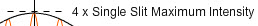
Figure 24: Double Slit Scale
13
Try 3, 4, and 5 slits. The bright fringes are much narrower, but their intensity is much greater. There are also some new smaller secondary maxima which occur where light from only some of the slits interfere constructively. Our full-brightness fringes are called principle maxima. At these locations, the light from all the slits interferes constructively.