
Chapter 2 – Quantum Theory
Introduction
Quantum theory explains our world at the atomic and molecular levels. A few brilliant scientists, who were trying to explain the results of experiments that defied the physics of the day, launched a theory that would change our view of not only the atom and the molecule, but of the universe as well. In this chapter, some of the key experiments leading to quantum theory are described, and then the theory is applied to the electrons in an atom.2.1 The Nature of Light
Introduction
Although we do not see atoms and molecules, much of our understanding of them is based on the way they interact with light. This lesson deals with the nature of light.Objectives
-
•Describe the relationship between the speed, wavelength, and frequency of a light wave.
-
•Determine the relative wavelengths and frequencies of two light waves given the region of the electromagnetic spectrum in which they lie.
2.1-1. Wavelength
Light is electromagnetic radiation; that is, it is an oscillating electric and magnetic field that travels through space at a constant speed,c = 2.998 × 10⁸ m/s,
the speed of light. The electric and magnetic fields are perpendicular to one another, but only the electric field is shown in the figures in this section.
A light wave is characterized by its amplitude, which is the distance between the valley and the peak of the wave, and its wavelength, λ, which is the distance between two adjacent maxima or minima in the electric (or magnetic) field. The amplitude indicates the brightness of the light, and the wavelength tells us what kind of light it is.
Visible light, the light visible to the human eye, is only a small fraction of all electromagnetic radiation, and the different colors that we see differ because they have different wavelengths. Red light has the longest wavelength in the visible region and violet light has the shortest.

Figure 2.1a: A 2800-nm Segment of Red Light
Red light has the longest wavelength of visible light. The red wave shown here has a wavelength of 700 nm. The 2800-nm segment contains four wavelengths of red light.

Figure 2.1b: A 2800-nm Segment of Violet Light
Violet light has the shortest wavelength of visible light. The violet wave shown here has a wavelength of 400 nm. The 2800-nm segment contains seven wavelengths of violet light.
2.1-2. Frequency
The product of the wavelength and frequency of a light wave equals the speed of light.
2.1-3. Electromagnetic Spectrum
An electromagnetic spectrum is a display of the component colors of a light beam, separated by their wavelengths. Raindrops can sometimes separate the component colors of white light by their wavelengths to produce a rainbow, which is a display of the spectrum of white light. Because the colors all merge into one another continuously, the resulting spectrum is called a continuous spectrum. A continuous spectrum can also be obtained by dispersing white light through a prism or from a grating. It should be noted that the visible region of the electromagnetic spectrum (that portion the eye can perceive) is but a small part of the entire spectrum. Further information about the EM spectrum can be found at http://imagine.gsfc.nasa.gov/docs/science/know_l1/emspectrum.html.
Figure 2.2: The Electromagnetic (EM) Spectrum
The visible region (400 – 700 nm), which is a very small portion of the spectrum, is expanded.
2.2 Quantization
Introduction
In this lesson, we introduce the concept of quantization, i.e., that energy comes in small packets called quanta.Objectives
-
•Define the terms quantized and photon.
-
•Calculate the energy of a photon from its frequency.
-
•Explain what is meant by 'wave-particle duality.'
-
•Define continuous spectrum and describe the spectrum of white light.
-
•Use the Rydberg equation to determine the frequency of a spectral line from the quantum numbers of the levels involved.
Blackbody Radiation
2.2-1. Blackbody Radiation Experiment
All objects emit electromagnetic waves, and as their temperature increases, so too do the total intensity and the average frequency of the radiation. At sufficiently high temperatures, a significant portion of the radiation is in the visible region of the spectrum. For example, a burner in an electric oven emits invisible but warm infrared radiation on a low setting, but it becomes 'red hot' on a high setting as it emits both infrared and visible radiation. Similarly, the tungsten filament of a light bulb becomes 'white hot' because all of the colors in the visible region are being emitted. This emission of electromagnetic waves from a warm body is called blackbody radiation.2.2-2. Blackbody Radiation Explanation
A photon is a bundle of light energy, which is proportional to the frequency of the light.
h = 6.626 × 10⁻³⁴ J-s
is called Planck's constant. The amount of energy in a wave that contains n quanta (photons) is then the following.
Planck's model for the quantization of wave energy correctly accounted for blackbody radiation, but the only reason he could offer for proposing this remarkable behavior was that it worked.
2.2-3. Photon Energy Exercise
Exercise 2.1:
What are the energies of the following in Joules? Express small numbers with the e format, e.g., 1.23e-12.
a photon red with a frequency of 4.60e14 s–1
3.04796e-19___
The energy of a single photon is 
E = hν = (6.626e−34 J s)(4.60e14 s−1) = 3.05e−19 J,
which is a very small amount of energy.
J
a mole of photons with frequency of 4.60e14 s–1
1.83548e5___
A mole of photons contains 6.02e23 electrons.
E = nhν = (6.02e23 mol−1)(6.626e−34 J s)(4.60e14 s−1) = 1.83e+5 J/mol = 183 kJ,
which is a substantial amount of energy.
J
The Photoelectric Effect
2.2-4. The Photoelectric Effect Experiment
Another observation of the late 1800s that could not be understood with the classical picture of light was that certain metals, when irradiated with light, ejected electrons. The kinetic energy of the electrons depended only upon the metal and the frequency of light. Increasing the intensity of the light increases the number of electrons that are ejected, but not their kinetic energy. For these metals, there is a minimum frequency below which no electrons are ejected, no matter how intense the light. This minimum frequency is called the threshold frequency of the metal, νo. As shown in Figure 2.3, a plot of the ejected electron's kinetic energy versus the frequency of the light striking the metal is a straight line.
Figure 2.3: Photoelectric Effect
No electrons are ejected when a metal is irradiated with light at frequencies below the threshold frequency (νo). At frequencies above the threshold frequency of the metal, electrons are ejected with a kinetic energy that increases linearly with the frequency of the light.
2.2-5. The Photoelectric Effect Explanation
In order to explain the photoelectric effect, Albert Einstein used Planck's hypothesis that light was composed of energy quanta. He proposed that light consisted of particles of energy, which we now call photons, each with an energy hν. He reasoned that, if the electrons are bound to a metal by an energy, W, then the threshold frequency for electron ejection from a metal (νo) is that frequency for whichhνo = W.
When the frequency (energy) of the photon is less than the threshold frequency of the metal, electrons cannot be removed because the energy that binds them to the metal is greater than the energy of the photon. However, when the energy of each photon exceeds the energy that binds the electron to the metal (hν > W),
the energy of the photon is transferred to the electron. A portion of the photon's energy, W, is used to overcome the potential energy binding the electron to the metal and the excess energy is converted into the kinetic energy of the ejected electron (KE).
According to Einstein, the intensity of a light wave reflects the number of photons that it contains. A beam that contains n photons has a total energy of nhν, but when light interacts with matter, it does so one photon at a time. Thus, it is the energy of each photon that dictates the energy of a molecular process that is initiated by the light, while the number of events that occur per unit time, i.e., the rate of the process is dictated by the intensity of the light.
Planck and Einstein had shown that light consisted of particles of energy called photons, but classical experiments showed that light is also a wave. This property of behaving as both a particle and a wave is called wave-particle duality.
Atomic Spectra
2.2-6. Continuous Spectrum
All wavelengths of visible light are present in white light, so when white light is dispersed as shown in Figure 2.4, the colors merge into one another continuously to produce a continuous spectrum.
Figure 2.4
2.2-7. Gas Discharge Tubes
A gas discharge tube is an evacuated tube that has been filled with a gas at low pressure. When high-energy electrons are passed through a discharge tube (a high voltage is placed across it), the tube glows with a color that is characteristic of the gas. As shown in Figure 2.5, a neon light has a characteristic red color, while a gas discharge tube filled with hydrogen glows with purple-blue color.
Figure 2.5
2.2-8. Line Spectra
Atomic spectra are line spectra.

Figure 2.6: Line Spectrum of Hydrogen
When the glow from a hydrogen discharge tube is focused down to the image of a slit and passed through a prism, it is broken down into four component wavelengths: 410 nm (violet), 434 nm (blue), 486 nm (green), and 656 nm (red). The four colors are observed as lines in the visible spectrum of hydrogen. However, there are over forty such lines observed throughout the ultraviolet, the visible, and the infrared.
-
1Look at Ne and compare the spectrum to the color of a neon light.
-
2Verify that Lithium has a strong line at 610 nm.
-
3Examine the spectra of the alkali metals. What general statement can be made about how the spectra of the atoms change as you proceed down a group?
2.2-9. Calculating the Line Spectrum of Hydrogen
Scientists did not understand the origin of line spectra, but Johannes Rydberg found a relatively simple mathematical expression, called the Rydberg equation and shown as Equation 2.3a below, that allowed him to calculate the frequency of every line in the hydrogen spectrum (over 40 lines). Multiplication of frequency in the Rydberg equation by Planck's constant yields the energy of the emitted photon in joules(E = hν)
as shown in Equation 2.3b.
-
•ν is the frequency of the emitted photon in s–1.
-
•Ephoton is the energy of the emitted photon with frequency ν.
-
•nlo < nhiare positive integers.
-
•RH = 3.290 × 10¹⁵ s−1is the Rydberg constant for hydrogen.
2.2-10. Rydberg Exercise
Exercise 2.2:
Use Equation 2.3a
ν = RH
−
= 3.290 × 10¹⁵
−
s−1
to determine the frequencies and wavelengths of the following spectral lines. Indicate whether each line falls in the infrared, visible, or ultraviolet region of the electromagnetic spectrum.
 |
| 1 |
| nlo2 |
| 1 |
| nhi2 |
 |
|
| 1 |
| nlo2 |
| 1 |
| nhi2 |
|
nlo = 2, nhi = 4
ν =
6.16875e14___
Use the Rydberg equation to calculate the frequency (ν).
ν = 3.290 × 10¹⁵
−
= 6.169 × 10¹⁴ s−1
s–1
|
| 1 |
| 22 |
| 1 |
| 42 |
|
nlo = 2, nhi = 4
λ =
485.998___
Use
c = λν
to calculate the wavelength (λ).
λ = cν =
= 4.860 × 10⁻⁷ m = 486.0 nm
nm
| 2.998 × x 108 m |
| 6.169 × 10¹⁴ s−1 |
-
nlo = 2, nhi = 4 region:
-
infrared
-
visible 486 nm is in the visible region. This is the blue-green line in the atomic spectrum of H. nlo = 2 for all of the lines in visible region of the hydrogen spectrum.
-
ultraviolet
nlo = 1, nhi = 2
ν =
2.4675e15___
Use the Rydberg equation to calculate the frequency (ν).
ν = 3.290 × 10¹⁵
−
= 2.468 × 10¹⁵ s−1
s–1
|
| 1 |
| 12 |
| 1 |
| 22 |
|
nlo = 1, nhi = 2
λ =
121.499___
Use
c = λν
to calculate the wavelength (λ).
λ = cν =
= 1.215 × 10⁻⁷ m = 121.5 nm
nm
| 2.998 × 10⁸ m |
| 2.468 × 10¹⁵ s−1 |
-
nlo = 1, nhi = 2 region:
-
infrared
-
visible
-
ultraviolet 121.5 nm is in the ultraviolet region. nlo = 1 for all of the lines in the ultraviolet region of the hydrogen spectrum.
nlo = 4, nhi = 7
ν =
1.38482e14___
Use the Rydberg equation to calculate the frequency (ν).
ν = 3.290 × 10¹⁵
−
= 1.385 × 10¹⁴ s−1
s–1
|
| 1 |
| 42 |
| 1 |
| 72 |
|
nlo = 4, nhi = 7
λ =
2164.900___
Use
c = λν
to calculate the wavelength (λ). λ = cν =
= 2.165 × 10⁻⁶ m = 2165 nm
nm
| 2.998 × 10⁸ m |
| 1.385 × 10¹⁴ s−1 |
-
nlo = 4, nhi = 7 region:
-
infrared 2165 nm is in the infrared region. All lines in which nlo = 4 are in the infrared. The lines with nlo = 5 are also in the infrared.
-
visible
-
ultraviolet
2.3 Bohr Model
Introduction
In the Rutherford model, electrons moved in circular orbits, but particles tend to move in straight lines not circles, so circular orbits require a force, called the centripetal force, to pull the orbiting particle toward the center. Earth is kept in its orbit by the gravitational attraction of the sun, and the electron is kept in its orbit by the Coulombic attraction of the nucleus. However, there was one major flaw with these orbiting electrons: the orbit would be unstable because a charged particle moving in this way would radiate energy, which would cause it to spiral into the nucleus, but clearly that was not the case in the hydrogen atom!Prerequisites
-
•1.8 Electromagnetism and Coulomb's Law (Relate the energy of interaction between two charged particles to the distance separating them.)
Objectives
-
•Relate energy of an electron to its n quantum number and the nuclear charge.
-
•Draw an energy level diagram for the hydrogen atom that shows the relative separations between the energy levels.
2.3-1. Bohr Radius
Note that the discussions of this section all ignore interactions between electrons, so they pertain only to systems that involve a single electron interacting with a nucleus with Z protons. Thus, the discussions are relevant to a H atom
(Z = 1),
but they do not apply to other atoms because all other atoms contain more than one electron. However, they do apply to the one-electron ions of other atoms such as He1+, Li2+, Be3+, etc.
(n = 1,2,3,4,  ).
).
By forbidding ).n = 0,
he assured that the electron always had some angular momentum, which stabilized the orbit and kept the electron moving in its circular path! He used Coulomb's Law to evaluate the electron-nuclear attraction (Fe in Figure 2.7) and the quantized angular momentum to determine the centripetal force (Fc in Figure 2.7). He then equated the two forces to determine the stable radii of rotation to be the following.
The n2 dependence expressed of the radius that appears in the equation is shown in Figure 2.7. The constant (52.92 pm) was calculated from known physical constants, such as Planck's constant, and the mass and charge of the electron and the proton. Z is the atomic number (number of positive charges in the nucleus). For a hydrogen atom, n = 1 and Z = 1,
so the distance between the electron and the proton was determined to be r1 = 52.92 pm,
which is called the Bohr radius.

Figure 2.7: Relative Radii of First Four Bohr Orbits
r1 = 52.92 pm, and rn = n2r1
2.3-2. Electron Energy
The energy of an electron in an atom is quantized, so electrons are said to occupy energy levels.
E = KE + U.
The potential energy of the electron in a one-electron system arises from its Coulombic energy of interaction with the nucleus, and its kinetic energy from its circular motion about the nucleus. However, the fact that the centripetal force resulted from the Coulombic force required that the kinetic energy be one-half of the Coulombic energy but opposite in sign (i.e., KE = −1/2U).
The total energy is then E = KE + U = −1/2U + U = 1/2U.
The Coulombic energy of interaction between the nucleus and the electron is given by Coulomb's Law (Equation 1.2), so the total energy of an electron in the nth orbit is the following.
The basic unit of charge is q = 1.602 × 10⁻¹⁸ C,
so the charge on an electron is qe = −q
and the charge on a nucleus with Z protons is qN = +Zq.
The value of ε in a vacuum is one, and r is the radius of the nth orbit as given in Equation 2.4rn = (5.292 × 10⁻¹¹)
m = (52.92)
pm
. Substitution of these known quantities into the preceding energy expression yields the total energy of an electron in the nth orbit in terms of the n quantum number.
The constant determined by Bohr, |
| n2 |
| z |
|
|
| n2 |
| z |
|
2.180 × 10⁻¹⁸ J,
was the same as the experimental value determined by Rydberg for hRH in Equation 2.3bEphoton = hν = hRH =
−
= 2.180 × 10⁻¹⁸
−
J
(i.e., |
| 1 |
| nlo2 |
| 1 |
| nhi2 |
|
|
| 1 |
| nlo2 |
| 1 |
| nhi2 |
|
2.180 × 10−18 = hRH).
This agreement with experiment was strong support for the Bohr model.
The energy associated with each value of n in Equation 2.5 is called an energy level. In the case of a hydrogen atom, Z = 1,
so the energy of the n = 1
level is –2.180 × 10⁻¹⁸ J, and that of the n = 2
level is −2.180 × 10⁻¹⁸(12/22) = −5.450 × 10⁻¹⁹ J.
The energies are negative because the energy of an electron in an atom is less than that of a free electron.
2.3-3. Bohr Model Exercise
Exercise 2.3:
Use the Bohr model to determine the orbtial radius and energy of an electron in the
n = 1
level of a Li2+ ion. We use the +2 ion because the Bohr model only applies to species with one electron.
Z =
3_0__
Li has three protons in its nucleus.
n =
1_0__
n = 1 is given in the problem.
rn =
17.64___
Use Equation 2.4:
rn = 52.92(12/3) = 17.6 pm
pm
En =
-1.962e-17___
Use Equation 2.5:
En = −2.180 × 10⁻¹⁸(32/12) = −1.962 × 10⁻¹⁷ J
J
2.3-4. Energy Level Diagram
Atomic spectra can be understood in terms of the electron moving from one energy level into another, which is referred to as an electronic transition. If nhi is the higher quantum number and nlo is the lower quantum number, then the energy difference between the two energy levels isΔE = Enhi − Enlo,
which can be determined with Equation 2.5En = (−2.180 × 10⁻¹⁸)
J = (−hRH)
to be the following.
ΔEatom in Equation 2.6 is identical to Ephoton in the empirical Equation 2.3b |
| Z2 |
| n2 |
|
|
| Z2 |
| n2 |
|
Ephoton = hν = hRH =
−
= 2.180 × 10⁻¹⁸
−
J
. Thus, an electron's energy can change by ΔEatom
by either absorbing of emitting a photon with an energy of Ephoton.
|
| 1 |
| nlo2 |
| 1 |
| nhi2 |
|
|
| 1 |
| nlo2 |
| 1 |
| nhi2 |
|
-
•Absorption: a photon is absorbed if nlo is the initial level. The absorption of energy increases the energy of the electron to the level of nhi.
-
•Emission: a photon is emitted if nhi is the initial level. The emission of energy decreases the energy of the electron to the level of nlo.
nlo = 2 and nhi = 3,
which is designated as the n = 3 to n = 2
transition (3 → 2). The violet line in the H atom spectrum is the highest energy line in the visible region; it results from the 6 → 2 transition. Note that the lines would correspond to absorptions if the arrows were pointed in the opposite direction. For example, the 2 → 3 transition is an absorption because the initial level is nlo. Note the following for hydrogen atom spectrum:
-
•nlo = 1 for all lines in the ultraviolet region.
-
•nlo = 2 for all lines in the visible region.

Figure 2.8: Energy Level Diagram for Hydrogen
2.3-5. Color
In a gas discharge tube, a high energy electron collides with an atom and transfers some of its energy to an electron in the atom, exciting the electron into a higher energy level (energy is absorbed). However, electrons always seek the lowest energy level, so the excited electron soon returns to a lower energy level. When it does so, it must give up all or some of the energy that it absorbed initially. Many of the electrons that are excited in this manner give up their energy by emitting photons. Only a fraction of the emitted photons fall in the visible region of the spectrum, but they are the ones that produce the glow in the tube. Light is a form of energy that results from changes that occur during atomic and molecular processes, and its frequency depends upon the type of process. For example, molecules absorb microwave radiation when they rotate, and they absorb infrared radiation when their atoms vibrate back and forth against their bonds. Visible light originates in electronic transitions; all color is the result of these transitions. A red shirt appears red because it reflects the red portion of white light and absorbs the green portion. The fabric of the shirt contains dye molecules that have electrons that absorb green light when they undergo electronic transitions between energy levels. The levels, however, are not separated by an energy equal to the energy of red photons, so the red photons are reflected and not absorbed. Our eyes perceive the reflected red photons but not the green ones that are absorbed by the shirt.2.4 Quantum Theory
Introduction
The theory that explains blackbody radiation, the photoelectric effect, and line spectra is called quantum theory. Quantum theory completely changed the way we think about matter. This lesson completes our study of the evolution of chemical theory from Lavoisier's introduction of elements and compounds to where it is today.Objectives
-
•Explain what is meant by electron density and why it is used instead of electron position.
2.4-1. Vibrating Strings
The reason behind quantization was the cause of much discussion, and the answer was finally presented by a graduate student in his Ph.D. thesis. Louis deBroglie recognized a similarity between the behavior of electrons and that of a vibrating string! Plucking a string of length L that is tied at both ends produces standing waves as shown in Figure 2.9. Since the string is tied down at each end, there must be an integral number of half-wavelengths in the distance L, i.e., the wavelength of each wave (λ) must obey the relationshipL = n × (λ/2) or λ = 2L/n.
The various values of the integer n define the harmonics. Note that L = 0
(no string) when n = 0,
so n cannot be zero. This is analogous to the Bohr model where the n quantum number is a positive, nonzero integer.
The points where the waves have zero amplitude are called nodes (indicated by arrows for n = 2 and n = 3).
Each wave has (n – 1) nodes, not counting the two ends.

Figure 2.9: Standing Waves in a Vibrating String
If the length of the string is L, then the wavelength of each wave is λ = 2L/n, where n is a nonzero integer. The number of nodes, points of zero amplitude, present in each wave as dictated by the red arrows is n – 1.
2.4-2. Quantum Theory
Electrons can behave as either particles or waves.
2.5 The Quantum Numbers
Introduction
Electrons must be treated like waves in modern quantum theory, and their full description requires four numbers called quantum numbers. In this section, we identify the four quantum numbers for an electron in an atom and explain the relationships between them.Objectives
-
•State the restrictions on each of the quantum numbers.
-
•Indicate the information available from each quantum number.
-
•Differentiate between an acceptable and unacceptable sets of quantum numbers and correct unacceptable sets.
-
•Give the letter used to describe each value of the l quantum number.
-
•Indicate the relative energies of several sublevels given their n and l quantum numbers.
2.5-1. Quantum Numbers and Orbital Energy Video
- Viewing the Video
-
•View the video in this window by selecting the play button.
-
•Use the video controls to view the video in full screen.
-
•View the video in text format by scrolling down.
-
•Jump to the exercises for this topic.
2.5-2. Introduction
Four quantum numbers are required for the complete description of an electron in an atom.
2.5-3. n Quantum Number
The n quantum number dictates the energy level of the electron.
-
•The principal quantum number dictates the energy level of the electron, so it is the primary, but not sole indicator of the electron's energy.
-
•n also indicates the average distance from the nucleus. On the average, electrons with high n quantum numbers are farther from the nucleus than those with lower n quantum numbers.
-
•Restrictions on n: n must be a nonzero, positive integer, i.e.,n = 1, 2, 3, , ∞.
2.5-4. l Quantum Number
The n and l quantum numbers determine an electron's sublevel, which determines the electron's energy.
-
•n and l define the sublevel. The energy of the electron depends upon the sublevel it occupies.
-
•Restrictions on l: l is an integer such that0 ≤ l < nin any sublevel.
-
•There are n sublevels in each level. For example, ifn = 3level, then l can be 0, 1, or 2 for a total of three sublevels.
| l quantum number | letter designation |
| 0 | s |
| 1 | p |
| 2 | d |
| 3 | f |
Note: the letters are derived from the appearance of the lines in an atomic line spectrum: s = sharp, p = principle, d = diffuse, f = fundamental. Sublevels with
l > 3
are labeled in order as g, h, i, ....
2.5-5. ml Quantum Number
n, l, and ml specify the electron's orbital.
-
•n, l, and ml specify the orbital.
-
•l and ml dictate the shape of the orbital, while n defines its size.
-
•Restrictions: the allowed values of ml depend upon the sublevel.−l ≤ ml ≤ +l,so there are 2l + 1 orbitals in a sublevel.
n = 3
level shown in Figure 2.10, where each line represents one orbital. Because n = 3,
there are three sublevels: l = 0, 1, and 2,
which correspond to the 3s, 3p and 3d sublevels, respectively. In an l = 0
sublevel, there can be only one value of ml and, therefore, only one orbital (ml = 0).
This is the 3s orbital. In an l = 1
sublevel, there are three allowed values of ml (–1, 0, +1) and, consequently, three orbitals. These three orbitals are the 3p orbitals. In the l = 2 sublevel, ml = −2, −1, 0, +1, and +2
for the five orbitals in the 3d sublevel. Thus, in the n = 3
level, there are three sublevels and nine orbitals.

Figure 2.10: Sublevels and Orbitals of the n = 3 Level
2.5-6. ms Quantum Number
ms determines the electron's spin. All magnetic fields are due to spin.
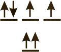
Classical Picture of Electron Spin: The two values of ms are represented with arrows.
- Viewing the Video
-
•View the video in this window by selecting the play button.
-
•Use the video controls to view the video in full screen.
-
•View the video in text format by scrolling down.
-
•Jump to the exercises for this topic.
ms = +1/2 and ms = −1/2.
All magnetic properties are attributed to electron spin, so it is often represented as the spin of the electron about its own axis in a clockwise (ms = +1/2)
or counterclockwise (ms = −1/2)
direction because a magnetic field is produced by a charge moving in a circular path. Thus, the 'spinning charge' can be thought to generate a magnetic field as indicated by the arrows in Figure 2.11. The arrow representing the magnetic field is often used to represent the ms quantum number of the electron. An up arrow ('up spin') is used to indicate an electron with ms = +1/2
and a down arrow ('down spin') indicates an electron with ms = −1/2.

Figure 2.11
The two values of ms are represented with up or down arrows.
2.5-7. Energy Levels and Quantum Numbers
Sublevels are named by giving the n quantum number followed by the letter that designates the l quantum number.
n = 3 and l = 2
is referred to as the 3d sublevel.
The relative energies of the sublevels can be determined from the following:
-
•They increase with the value of (n + l) for the sublevel.
-
•The energies of sublevels with the same value of (n + l) increase with increasing n.
2.5-8. Quantum Number Exercise
Exercise 2.4:
What are the n and l quantum numbers for a 6f electron?
n =
6_0__
The number is the n quantum number, so
n = 6
.
l =
3_0__
The letter designates the l quantum number. f is used to designate an
l = 3
sublevel.
What is the designation of each of the following sublevels?
n = 3, l = 2
o_3d_ins
l = 2 is a d sublevel.
n = 5, l = 1
o_5p_ins
l = 1 is a p sublevel.
n = 6, l = 3
o_6f_ins
l = 3 is an f sublevel.
n = 4, l = 0
o_4s_ins
l = 0 is an s sublevel.
How many sublevels are in an n = 4 level?
4_0__
The l quantum number can be any integer from 0 to (n – 1), inclusively. Note it cannot equal n. Therefore, the allowed values of l in the n = 4 level are 0, 1, 2, and 3. There are four sublevels in the n = 4 level. Note that there are always n sublevels in the nth level.
-
Which sublevel is at lower energy?
-
4s The lower energy sublevel is the one with the lower value of (n + l).
- For a 4s sublevel, n = 4, and l = 0;, so n + l = 4
- For a 3d sublevel, n = 3 and l = 2;, so n + l = 5
-
3d
-
Which sublevel is at lower energy?
-
4p
-
3d The lower energy sublevel is the one with the lower value of (n + l).
- For a 4p sublevel, n = 4, and l = 1;, so n + l = 5
- For a 3d sublevel, n = 3 and l = 2;, so n + l = 5
2.5-9. Quantum Number Restrictions Exercise
Exercise 2.5:
The following sets of quantum numbers are not valid but can be made so by correcting one value. Identify the invalid quantum number as n, l, ml, or ms in each and supply an acceptable value. If there is more than one acceptable value enter the lowest, positive value or zero.
-
n = 3, l = 3, ml = –3, ms = +1/2
-
n l must be less than n, but ml cannot exceed l.
-
l
-
ml
-
ms
invalid number:
-
n = 75, l = 74, ml = 0, ms = 0
-
n
-
l
-
ml
-
ms There are only two possible spins.
invalid quantum number:
acceptable value
4_0__
n can be any integer greater than 3, so the lowest acceptable value is 4.
acceptable value
o_+1/2_s
Either +1/2 or –1/2 is acceptable.
-
n = 6, l = –5, ml = –5, ms = –1/2
-
n
-
l l cannot be negative.
-
ml
-
ms
invalid quantum number:
-
n = 2, l = 0, ml = 2, ms = +1/2
-
n
-
l
-
ml l cannot be less than ml, but it must be less than n.
-
ms
invalid quantum number:
acceptable value
5___
l must be less than n, but not less than the absolute value of ml.
acceptable value
0___
The absolute value of ml cannot be less than l.
2.6 Orbital Shapes and Sizes
Introduction
Orbitals are at the heart of chemistry because it is the interaction between orbitals that produces chemical bonds. Mathematically, an orbital is a wave function with specified values for n, l, and ml. Like other functions, they can be positive or negative, and the sign of the orbital will be important when we combine them to produce molecular orbitals in Chapter 6. In this section, we consider the shapes of only the s and p orbitals because they are the only orbital types that will be used in the next several chapters.Objectives
-
•Draw s orbitals.
-
•Draw p orbitals and define nodal planes.
2.6-1. s Orbitals
s orbitals are spherical and positive everywhere.

Figure 2.12: s Orbitals
The relative sizes of the 1s, 2s, and 3s orbitals of an atom
2.6-2. p Orbitals
p orbitals each contain a nodal plane.
l = 1
for p orbitals. There are three values of ml (–1, 0, +1), so there are three orbitals in a p sublevel. The three p orbitals are perpendicular to one another and are referred to as the px, py, and pz orbitals. The electron density in each p orbital lies along one of the cartesian axes, but each orbital contains a nodal plane, a plane of zero electron density that passes through the nucleus of the atom. The nodal plane is shown as a gray rectangle in Figure 2.13a. In general, the number of nodal planes in an orbital is equal to its l quantum number. l = 1
for p orbitals, so they each have one nodal plane.
The function that describes a p orbital is positive in one lobe, zero at the nodal plane, and negative in the other lobe. The fact that the sign of the orbital functions is different in the two lobes will be important in our discussion of bonding, and this point is often emphasized by the shading of the two lobes. We use blue and red to distinguish between the two. Blue will be used to identify lobes where the function is positive and red will be used for lobes in which the function is negative.

Figure 2.13a: p Orbitals: True Representation

Figure 2.13b: p Orbitals: Common "Figure 8" Representation
2.6-3. d Orbitals
d orbitals each contain two nodal planes.
l = 2
sublevel (–2, –1, 0, +1, +2), so there are five d orbitals. Figure 2.14 shows a representation of these orbitals. The dz2 (or simply z2) orbital is directed along the z-axis, but there is a donut shaped region of electron density in the xy-plane. The x2 – y2 orbital is directed along both the x- and the y-axes in both the positive and negative directions. Much of the dxz (xz) electron cloud lies in the xz-plane 45° from either axis. The shapes of the dyz (yz) and dxy (xy) are identical to that of the dxz, only the labels of the axes change.

Figure 2.14: d Orbitals
2.7 Electron Configurations
Introduction
The number of electrons in each sublevel is given by the electron configuration of an atom. Electron configurations, the topic of this section, will help us predict the bonding properties of an atom.Objectives
-
•Write an electron configuration from a sublevel population.
-
•Use the Pauli Exclusion Principle to distinguish between acceptable and unacceptable ways for electrons to occupy an orbital.
-
•Use Hund's Rule to determine a lowest energy electron configuration of an atom with a partially filled sublevel.
-
•Determine the lower energy configuration based on the sublevel populations of two different configurations
-
•Determine whether an arrangement of electrons represents a ground state, an excited state, or is not acceptable.
-
•Use an energy level diagram and the number of electrons in an atom to write the ground state electron configuration of the atom.
-
•Determine the number of unpaired electrons in an atom's ground state electron configuration.
-
•Write electron configurations using the noble gas core abbreviation.
-
•Write the electron configurations for the two elements in the fourth period that are exceptions to the trend in configurations.
2.7-1. Electron Configurations Video
- Viewing the Video
-
•View the video in this window by selecting the play button.
-
•Use the video controls to view the video in full screen.
-
•View the video in text format by scrolling down.
-
•Jump to the exercises for this topic.
2.7-2. Electron Configurations
An electron configuration specifies the occupied sublevels and the number of electrons in each.
-
•n is the n quantum number.
-
•l is the l quantum number of the sublevel expressed as a letter (s, p, d, ...).
-
•p is the sublevel population (i.e., the number of electrons in the sublevel).
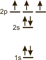
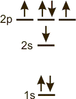
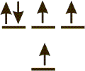
2.7-3. Pauli Exclusion Principle
No orbital can have more than one electron of a given spin, so no orbital can have more than two electrons.
(ms = +1/2)
and one with spin down (ms = −1/2).
Since, the two electrons in an orbital have opposite spins, they are said to be paired. An electron that occupies an orbital alone is said to be unpaired. Similarly, an orbital with two electrons is full, while an orbital with one electron is said to be half-filled.

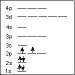
Figure 2.15: Pauli Exclusion Prinicple
A and B are acceptable, but C and D are not because they violate the Pauli Exclusion Principle.
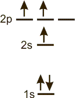
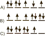
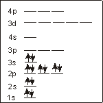
2.7-4. Hund's Rule
The lowest energy arrangement of electrons in an unfilled sublevel is the one that maximizes the number of electrons with identical spin.

Figure 2.16: Hund's Rule
A is the lowest energy configuration because it obeys Hund's Rule. The energies of B and C are greater than that of A because the three spins are not the same. B and C are excited states.
2.7-5. Lowest Energy Configurations
Electrons occupy the unfilled orbitals of lowest energy (i.e., the sublevels with the lowest value of n + l). Remember that the energies of sublevels with the same value of (n + l) increase in order of increasing n. Also recall that l cannot be greater than (n – 1). The order of sublevels in increasing energy through(n + l) = 7
is given below.
| order | n + l | n | l | sublevel | |
order | n + l | n | l | sublevel |
| 1 | 1 | 1 | 0 | 1s | |
9 | 5 | 5 | 0 | 5s |
| 2 | 2 | 2 | 0 | 2s | |
10 | 6 | 4 | 2 | 4d |
| 3 | 3 | 2 | 1 | 2p | |
11 | 6 | 5 | 1 | 5p |
| 4 | 3 | 3 | 0 | 3s | |
12 | 6 | 6 | 0 | 6s |
| 5 | 4 | 3 | 1 | 3p | |
13 | 7 | 4 | 3 | 4f |
| 6 | 4 | 4 | 0 | 4s | |
14 | 7 | 5 | 2 | 5d |
| 7 | 5 | 3 | 2 | 3d | |
15 | 7 | 6 | 1 | 6p |
| 8 | 5 | 4 | 1 | 4p | |
16 | 7 | 7 | 0 | 7s |
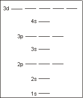
2.7-6. Sublevel Energy Diagram
Orbital energies increase with n + l. Orbitals with the same value of n + l increase in order of n.

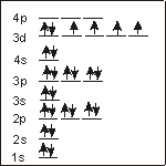
Figure 2.17: Atomic Orbitals in Order of Increasing Energy
2.7-7. Ground States
In the ground state configuration, there can be no unfilled orbitals lower in energy than the highest energy electron.
-
1the Pauli Exclusion Principle is obeyed.
-
2the occupied sublevels are those at lowest energy.
-
3Hund's Rule is obeyed.
2.7-8. Unpaired Electrons
The number of unpaired electrons in a sublevel is maximized by Hund's Rule.
-
1Ground state electron configuration: the listing of the occupied sublevels and their populations
-
2Unpaired electrons: Unpaired electrons exist in unfilled sublevels and their number is maximized by Hund's Rule. (As we will see in Chapter 3, the number of unpaired electrons is an important characteristic of the atom because it dictates the atom's magnetic properties.)
2.7-9. Using Noble Gas Cores in Electron Configurations
The electron configurations of the atoms become unwieldy as the number of electrons in the atom increases. For example, iodine's electron configuration is1s2 2s2 2p6 3s2 3p6 4s2 3d10 4p6 5s2 4d10 5p5
[Kr] 5s2 4d10 5p5
2.7-10. Electron Configuration Exercises
Exercise 2.6:
configuration:
configuration:
configuration:
Write the electron configuration of each of the following diagrams. Also indicate whether the configuration is ground state or an excited state configuration. (Separate all terms by a single space and indicate all superscripts with a carat (^). For example, 2s^2 2p^2 for 2s2 2p2.)
configuration:
o_1s^2 2s^1 2p^2_s
There are 2 electrons in the 1s sublevel, 1 in the 2s sublevel and 2 in the 2p sublevel, so the configuration is 1s2 2s1 2p2.
configuration:
o_1s^2 2s^2 2p^3_s
There are 2 electrons in the 1s sublevel, 1 in the 2s sublevel and 4 in the 2p sublevel, so the configuration is 1s2 2s1 2p4.
configuration:
o_1s^2 2s^1 2p^4_s
There are no unfilled orbitals at low energy, and Hund's Rule is obeyed.
-
ground state There are 2 electrons in the 1s sublevel, 2 in the 2s sublevel and 3 in the 2p sublevel, so the configuration is 1s2 2s2 2p3.
-
excited state
-
ground state
-
excited state The 2p is occupied, but the 2s is not yet full.
-
ground state The 2p is occupied, but the 2s is not yet full. Also, Hund's Rule is not obeyed.
-
excited state
2.7-11. Two Exceptions
Chromium and copper are the only two exceptions we deal with.
-
1Chromium promotes a 4s electron to attain an [Ar] 4s1 3d5, which has a half-filled 3d sublevel.
-
2Copper promotes a 4s electron to attain an [Ar] 4s1 3d10, which has a filled 3d sublevel.

Figure 2.18
Cr promotes a 4s electron to attain a half-filled 3d sublevel.

Figure 2.19
Cu promotes a 4s electron to attain a filled 3d sublevel.
2.7-12. Energy Level Exercise
Exercise 2.7:
Extend the energy level diagram for the sublevels to include
n + l = 6
and n + l = 7.
Place the lowest energy sublevel at the bottom (4d) and the highest energy sublevel at the top (7s). Include the number of orbitals in each.
sublevel 7s
orbitals
1___
There is one orbital in an s sublevel.
sublevel
o_6p_ins
n + l = 6 + 1
orbitals
3___
There are three orbitals in a p sublevel.
sublevel
o_5d_ins
n + l = 5 + 2
orbitals
5___
There are five orbitals in a d sublevel.
sublevel
o_4f_ins
n + l = 4 + 3
orbitals
7___
l = 3, so there are seven orbitals in an f sublevel.
sublevel
o_6s_ins
n + l = 6 + 0
orbitals
1___
There is one orbital in an s sublevel.
sublevel
o_5p_ins
n + l = 5 + 1
orbitals
3___
There are three orbitals in a p sublevel.
sublevel 4d
orbitals
5___
l = 2, so there are five orbitals in a d sublevel.
2.7-13. Shorthand Notation Exercise
Exercise 2.8:
Use the energy level diagram for the sublevels through
n + l = 5
in Figure 2.17 and the levels for n + l = 6 and 7
that were determined in the previous exercise to determine sublevel populations for the ground states of the following. Then use the noble gas core shorthand to write their electron configurations. Place a space after the noble gas and between each sublevel. The sublevel energies continue from those.
Rb
o_[Kr] 5s1_ins
The preceding noble gas is Kr, and Rb is the first member of the 5s block. Rubidium is [Kr] 5s1.
Sn
o_[Kr] 5s2 4d10 5p2_ins
The preceding noble gas is Kr. In addition, the 5s and 4d blocks are full and Sn is the second member of the 5p block. Tin is [Kr] 5s2 4d10 5p2 .
Bi
o_[Xe] 6s2 4f14 5d10 6p3_ins
The preceding noble gas is Xe. In addition, the 6s, 4f (between Z = 57 and Z = 72), and 5d blocks are full and Bi is the third member of the 6p block. Bismuth is [Xe] 6s2 4f14 5d10 6p3.
2.7-14. Hund's Rule Exercise
Exercise 2.9:
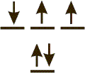
Which arrangement of d electrons has the lowest energy in each case?
-
A This arrangement has two electrons with 'spin up' and two electrons with 'spin down', so it does not maximize the number of electrons with the same spin.
-
B This arrangement has three spin-up electrons and one spin-down electron, which does not produce the maximum number of electrons with the same spin. It is a violation of Hund's Rule, so it is not the lowest energy arrangement.
-
C
-
D This arrangement has two spin-up electrons and two spin-down electron, which does not produce the maximum number of electrons with the same spin. It is a violation of Hund's Rule, so it is not the lowest energy arrangement.
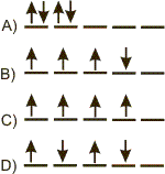
-
A This arrangement does not maximize the number of electrons with the same spin, so it does not obey Hund's Rule and is not the lowest energy arrangement.
-
B
-
C This arrangement maximizes the number of electron pairs not the number of electrons with the same spin. Thus, it does not obey Hund's Rule and does not have the lowest energy.
2.7-15. Indentifying States Exercise
Exercise 2.10:
Indicate whether each of the following represents a ground state, an excited state, or are unacceptable configuration. Assume that all sublevels at lower energy are filled.
-
ground state There is an unfilled sublevel at lower energy than an occupied sublevel, so this is not the ground state.
-
excited state The Pauli Exclusion Principle is obeyed, but there is an unfilled sublevel at lower energy than an occupied sublevel, so this is an excited state.
-
not acceptable All electrons obey the Pauli Exclusion Principle (no two electrons in the same orbital have the same spin), so it is an acceptable arrangement.
-
ground state This is not an acceptable ground state configuration.
-
excited state This is not an acceptable excited state.
-
not acceptable The two electrons in the 2s orbital have the same spin, so they have the same quantum numbers, which violates the Pauli Exclusion Principle. Consequently, this is an unacceptable configuration.
-
ground state This arrangement does not obey Hund's Rule, so it is not the ground state.
-
excited state This arrangement does obey the Pauli Exclusion Principle, so it is an acceptable arrangement. However, it does not obey Hund's Rule because one of the spins in the 2p is the opposite of the other two. Therefore, this arrangement is an excited state.
-
not acceptable All electrons obey the Pauli Exclusion Principle (no two electrons in the same orbital have the same spin), so it is an acceptable arrangement.
-
ground state This arrangement has no unfilled orbitals at lower energy than occupied orbitals and obeys both the Pauli Exclusion Principle and Hund's Rule, so it is the ground state.
-
excited state This arrangement has no unfilled orbitals at lower energy than occupied orbitals and obeys Hund's Rule, so it is not an excited state.
-
not acceptable All electrons obey the Pauli Exclusion Principle (no two electrons in the same orbital have the same spin), so it is an acceptable arrangement.
2.7-16. Unpaired Electrons Exercise
Exercise 2.11:
C (6 electrons):
configuration
o_1s2 2s2 2p2_ins
The Pauli Exclusion Principle states that there can be no more than two electrons per orbitals, so two electrons occupy the 1s, 2s, and 2p sublevels. The electron configuration of C is 1s2 2s2 2p2.
unpaired electrons
2___
Hund's Rule states that the electrons filling the 2p sublevel maintain the same spin and do not pair. Thus, there are two unpaired electrons in a carbon atom.
Hund's Rule states that the electrons filling the 2p sublevel maintain the same spin and do not pair. Thus, there are two unpaired electrons in a carbon atom.
Mg (12 electrons):
configuration
o_1s2 2s2 2p6 3s2_ins
Placing two electrons in each orbital in order of increasing energy, we obtain an electron configuration of 1s2 2s2 2p6 3s2.
unpaired electrons
0___
All of the occupied sublevels are full, so there are no unpaired electrons in a magnesium atom.
All of the occupied sublevels are full, so there are no unpaired electrons in a magnesium atom.
Fe (26 electrons):
configuration
o_1s2 2s2 2p6 3s2 3p6 4s2 3d6_ins
26 electrons fill the sublevels in order of increasing energy to produce the following electron configuration: 1s2 2s2 2p6 3s2 3p6 4s2 3d6.
unpaired electrons
4___
Only the 3d sublevel is unfilled, and Hund's Rule dictates that the number of electrons with the same spin in the unfilled sublevel must be maximized to produce four unpaired electrons.
Only the 3d sublevel is unfilled, and Hund's Rule dictates that the number of electrons with the same spin in the unfilled sublevel must be maximized to produce four unpaired electrons.
2.8 Quantum Theory and The Periodic Table
Introduction
Like other atomic properties, the electron configurations of the atoms are periodic. This periodicity allows us to determine the electron configuration of an atom from the atom's position in the periodic table.Objectives
-
•Write the electron configuration of an atom from its placement in the periodic table.
2.8-1. Periodicity of Electron Configurations Video
- Viewing the Video
-
•View the video in this window by selecting the play button.
-
•Use the video controls to view the video in full screen.
-
•View the video in text format by scrolling down.
-
•Jump to the exercises for this topic.
2.8-2. Electron Configurations and Periodicity
The sublevels fill in the following order (left to right then down).| 1s | |||
| 2s | 2p | ||
| 3s | 3p | ||
| 4s | 3d | 4p | |
| 5s | 4d | 5p | |
| 6s | 4f | 5d | 6p |
Each column represents the same type of sublevel (s, p, or d). The number of electrons required to fill each of these sublevels is
-
1s sublevel: 2 electrons.
-
2p sublevel: 6 electrons.
-
3d sublevel: 10 electrons.
| 1 2 | 1s | 1 2 3 4 5 6 |
| 2s | 2p | |
| 3s | 1 2 3 4 5 6 7 8 9 10 | 3p |
| 4s | 3d | 4p |
| 5s | 4d | 5p |
The above table has exactly the same form as the periodic table. If you understand this periodicity, you can determine the electron configuration of an atom from its position in the periodic table.
2.8-3. Periodic Table and Sublevels
s Block
Then = 1
level contains only one s sublevel. Thus, H and He are 1s1 and 1s2, respectively. However, their positions in the periodic table are normally not with the other elements of the s block. Hydrogen is often shown in the middle of the periodic table for reasons that will be explained in Chapter 4, and He is at the top of the Group 8A elements because it is a noble gas. The rest of the s block elements are those in Groups 1A and 2A. The n quantum number of the level to which the outermost sublevel belongs is given by the row number. Thus, the electron configurations of the outermost sublevel for the Group 1A and 2A elements are the following.
| 1A | 2A |
| ns1 | ns2 |
p Block
The elements of Groups 3A through 8A are filling a p sublevel. The n quantum number of the level to which the outermost sublevel belongs is given by the row number. Thus, the electron configurations of the outermost sublevel for the Group 3A through 8A elements have the following form.| 3A | 4A | 5A | 6A | 7A | 8A |
| np1 | np2 | np3 | np4 | np5 | np6 |
d Block
The elements of Groups 3B through 2B are filling a d sublevel. The n quantum number of the level to which the d sublevel belongs equals the row number – 1. Thus, elements scandium(Z = 21)
through zinc (Z = 30)
are filling the 3d sublevel, while yttrium (Z = 39)
through cadmium (Z = 48)
are filling the 4d sublevel.

Figure 2.20: s, p, d, and f Blocks in the Periodic Table
2.8-4. Table of Electron Configurations
Practice using the periodic table to predict the electron configuration of an atom. Check your answer by clicking on the element in the periodic table below.| 1 1A |
2 2A |
3 3B |
4 4B |
5 5B |
6 6B |
7 7B |
8 8B |
9 8B |
10 8B |
11 1B |
12 2B |
13 3A |
14 4A |
15 5A |
16 6A |
17 7A |
18 8A |
| H |
He |
||||||||||||||||
| Li |
Be |
B |
C |
N |
O |
F |
Ne |
||||||||||
| Na |
Mg |
Al |
Si |
P |
S |
Cl |
Ar |
||||||||||
| K |
Ca |
Sc |
Ti |
V |
Cr |
Mn |
Fe |
Co |
Ni |
Cu |
Zn |
Ga |
Ge |
As |
Se |
Br |
Kr |
| Rb |
Sr |
||||||||||||||||
2.8-5. Electron Configuration Exercise
Exercise 2.12:
Use the periodic table to help you write electron configurations for the following atoms. Use the Noble gas core abbreviation. (Separate all terms by a single space and indicate all superscripts with a carat (^). For example, [He] 2s^2 2p^2 for [He] 2s2 2p2.)
Sc
o_[Ar] 4s^2 3d^1_s
The electron configuration of scandium is [Ar] 4s2 3d1.
N
o_ [He] 2s^2 2p^3_s
The electron configuration of nitrogen is [He] 2s2 2p3.
Cu
o_[Ar] 4s^1 3d^10_s
Remember that copper is one of the exceptions because it promotes an s electron to fill the d sublevel. The electron configuration of copper is [Ar] 4s1 3d10.
Bi
o_[Xe] 6s^2 4f^14 5d^10 6p^3_s
The 4f block is filled, so the electron configuration of bismuth is [Xe] 6s2 4f14 5d10 6p3.
K
o_[Ar] 4s^1_s
Potassium is [Ar] 4s1.
Co
o_[Ar] 4s^2 3d^7_s
Cobalt is [Ar] 4s2 3d7.